
2.2 Perfect Competition and Supply and Demand
Under a mixed economy, such as we have in the United States, businesses make decisions about which goods to produce or services to offer and how they are priced. Because there are many businesses making goods or providing services, customers can choose among a wide array of products. The competition for sales among businesses is a vital part of our economic system. Economists have identified four types of competition—perfect competition, monopolistic competition, oligopoly, and monopoly. We’ll introduce the first of these—perfect competition—in this section and cover the remaining three in the following section.
Perfect Competition
exists when there are many consumers buying a standardized product from numerous small businesses. Because no seller is big enough or influential enough to affect price, sellers and buyers accept the going price. For example, when a commercial fisher brings his fish to the local market, he has little control over the price he gets and must accept the going market price.
The Basics of Supply and Demand
To appreciate how perfect competition works, we need to understand how buyers and sellers interact in a market to set prices. In a market characterized by perfect competition, price is determined through the mechanisms of supply and demand. Prices are influenced both by the supply of products from sellers and by the demand for products by buyers.
To illustrate this concept, let’s create a supply and demand schedule for one particular good sold at one point in time. Then we’ll define demand and create a demand curve and define supply and create a supply curve. Finally, we’ll see how supply and demand interact to create an equilibrium price—the price at which buyers are willing to purchase the amount that sellers are willing to sell.
Demand and the Demand Curve
is the quantity of a product that buyers are willing to purchase at various prices. The quantity of a product that people are willing to buy depends on its price. You’re typically willing to buy less of a product when prices rise and more of a product when prices fall. Generally speaking, we find products more attractive at lower prices, and we buy more at lower prices because our income goes further.
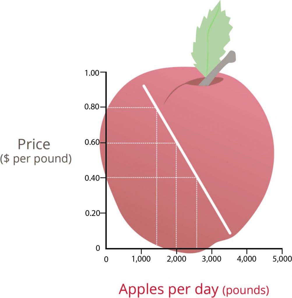
Using this logic, we can construct a demand curve that shows the quantity of a product that will be demanded at different prices. Let’s assume that the diagram in Figure 2.3 “” represents the daily price and quantity of apples sold by farmers at a local market. Note that as the price of apples goes down, buyers’ demand goes up. Thus, if a pound of apples sells for $0.80, buyers will be willing to purchase only fifteen hundred pounds per day. But if apples cost only $0.60 a pound, buyers will be willing to purchase two thousand pounds. At $0.40 a pound, buyers will be willing to purchase twenty-five hundred pounds.
Supply and the Supply Curve
is the quantity of a product that sellers are willing to sell at various prices. The quantity of a product that a business is willing to sell depends on its price. Businesses are more willing to sell a product when the price rises and less willing to sell it when prices fall. Again, this fact makes sense: businesses are set up to make profits, and there are larger profits to be made when prices are high.
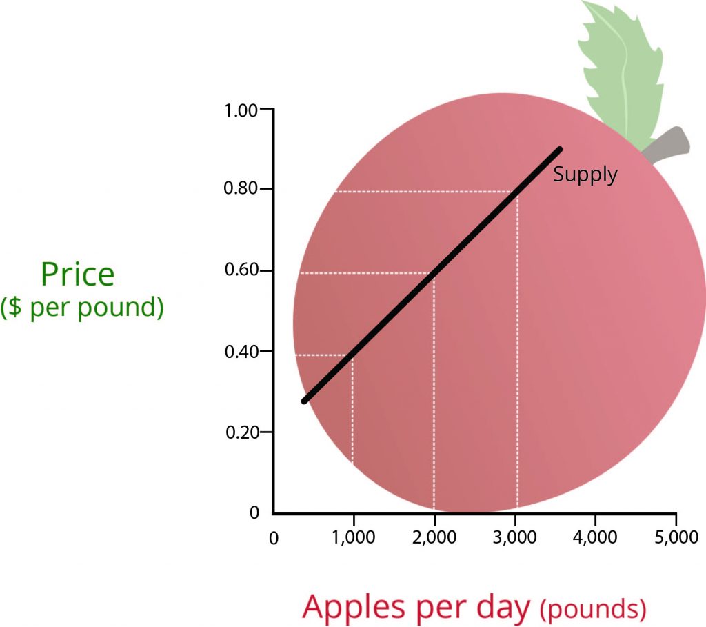
Now we can construct a supply curve that shows the quantity of apples that farmers would be willing to sell at different prices, regardless of demand. As you can see in Figure 2.4 “”, the supply curve goes in the opposite direction from the demand curve: as prices rise, the quantity of apples that farmers are willing to sell also goes up. The supply curve shows that farmers are willing to sell only a thousand pounds of apples when the price is $0.40 a pound, two thousand pounds when the price is $0.60, and three thousand pounds when the price is $0.80.
Equilibrium Price
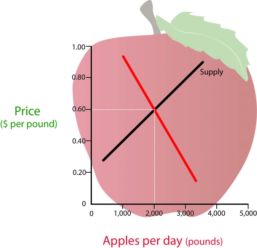
We can now see how the market mechanism works under perfect competition. We do this by plotting both the supply curve and the demand curve on one graph, as we’ve done in Figure 3.5 “The Equilibrium Price”. The point at which the two curves intersect is the .
You can see in Figure 2.5 “The Equilibrium Price” that the supply and demand curves intersect at the price of $0.60 and quantity of two thousand pounds. Thus, $0.60 is the equilibrium price: at this price, the quantity of apples demanded by buyers equals the quantity of apples that farmers are willing to supply. If a single farmer tries to charge more than $0.60 for a pound of apples, he won’t sell very many because other suppliers are making them available for less. As a result, his profits will go down. If, on the other hand, a farmer tries to charge less than the equilibrium price of $0.60 a pound, he will sell more apples but his profit per pound will be less than at the equilibrium price. With profit being the motive, there is no incentive to drop the price.
What have we learned in this discussion? Without outside influences, markets in an environment of perfect competition will arrive at an equilibrium point at which both buyers and sellers are satisfied. But we must be aware that this is a very simplistic example. Things are more complex in the real world. For one thing, markets don’t always operate without outside influences. For example, if a government set an artificially low price ceiling on a product to keep consumers happy, we would not expect producers to produce enough to satisfy demand, resulting in a . If government set prices high to assist an industry, sellers would likely supply more of a product than buyers need; in that case, there would be a .
Circumstances also have a habit of changing. What would happen, for example, if incomes rose and buyers were willing to pay more for apples? The demand curve would change, resulting in an increase in equilibrium price. This outcome makes intuitive sense: as demand increases, prices will go up. What would happen if apple crops were larger than expected because of favorable weather conditions? Farmers might be willing to sell apples at lower prices rather than letting part of the crop spoil. If so, the supply curve would shift, resulting in another change in equilibrium price: the increase in supply would bring down prices.
Key Takeaways
- There are three other types of competition in a free market system: monopolistic competition, oligopoly, and monopoly.
- In monopolistic competition, there are still many sellers, but products are differentiated, e., differ slightly but serve similar purposes. By making consumers aware these differences, sellers exert some control over price.
- In an oligopoly, a few sellers supply a sizable portion of products in the market. They exert some control over price, but because their products are similar, when one company lowers prices, the others follow.
- In a monopoly, there is only one seller in the market. The “market” could be a specific geographical area, such as a city. The single seller is able to control prices.
- All economies share three goals: growth, high employment, and price stability.
- To get a sense of where the economy is headed in the future, we use statistics called economic indicators. Indicators that report the status of the economy a few months in the past are lagging Those that predict the status of the economy three to twelve months in the future are called leading indicators.
when there are many consumers buying a standardized product from numerous small businesses
is the quantity of a product that buyers are willing to purchase at various prices
represents the daily price and quantity of apples sold by farmers at a local market
quantity of a product that sellers are willing to sell at various prices
graphic representation of the correlation between the cost of a good or service and the quantity supplied for a given period
The point at which the two curves intersect
When producers do not produce enough to satisfy demand
When sellers would likely supply more of a product than buyers need
