
Part 3: Using quantitative methods
15. Bivariate analysis
Chapter Outline
- What is bivariate data analysis? (5 minute read)
- Chi-square (4 minute read)
- Correlations (5 minute read)
- T-tests (5 minute read)
- ANOVA (6 minute read)
Content warning: examples in this chapter include discussions of anxiety symptoms.
So now we get to the math! Just kidding. Mostly. In this chapter, you are going to learn more about , or analyzing the relationship between two variables. I don’t expect you to finish this chapter and be able to execute everything you just read about—instead, the big goal here is for you to be able to understand what bivariate analysis is, what kinds of analyses are available, and how you can use them in your research.
Take a deep breath, and let’s look at some numbers!
15.1 What is bivariate analysis?
Learning Objectives
Learners will be able to…
- Define bivariate analysis
- Explain when we might use bivariate analysis in social work research
Did you know that ice cream causes shark attacks? It’s true! When ice cream sales go up in the summer, so does the rate of shark attacks. So you’d better put down that ice cream cone, unless you want to make yourself look more delicious to a shark.

Ok, so it’s quite obviously not true that ice cream causes shark attacks. But if you looked at these two variables and how they’re related, you’d notice that during times of the year with high ice cream sales, there are also the most shark attacks. Despite the fact that the conclusion we drew about the relationship was wrong, it’s nonetheless true that these two variables appear related, and researchers figured that out through the use of bivariate analysis. (For a refresher on correlation versus causation, head back to Chapter 8.)
consists of a group of statistical techniques that examine the relationship between two variables. We could look at how anti-depressant medications and appetite are related, whether there is a relationship between having a pet and emotional well-being, or if a policy-maker’s level of education is related to how they vote on bills related to environmental issues.
Bivariate analysis forms the foundation of multivariate analysis, which we don’t get to in this book. All you really need to know here is that there are steps beyond bivariate analysis, which you’ve undoubtedly seen in scholarly literature already! But before we can move forward with multivariate analysis, we need to understand whether there are any relationships between our variables that are worth testing.
A study from Kwate, Loh, White, and Saldana (2012) illustrates this point. These researchers were interested in whether the lack of retail stores in predominantly Black neighborhoods in New York City could be attributed to the racial differences of those neighborhoods. Their hypothesis was that race had a significant effect on the presence of retail stores in a neighborhood, and that Black neighborhoods experience “retail redlining”—when a retailer decides not to put a store somewhere because the area is predominantly Black.
The researchers needed to know if the predominant race of a neighborhood’s residents was even related to the number of retail stores. With bivariate analysis, they found that “predominantly Black areas faced greater distances to retail outlets; percent Black was positively associated with distance to nearest store for 65 % (13 out of 20) stores” (p. 640). With this information in hand, the researchers moved on to multivariate analysis to complete their research.
Statistical significance
Before we dive into analyses, let’s talk about statistical significance. is the extent to which our statistical analysis has produced a result that is likely to represent a real relationship instead of some random occurrence. But just because a relationship isn’t random doesn’t mean it’s useful for drawing a sound conclusion.
We went into detail about statistical significance in Chapter 5. You’ll hopefully remember that there, we laid out some key principles from the American Statistical Association for understanding and using p-values in social science:
- P-values can indicate how incompatible the data are with a specified statistical model. P-values can provide evidence against the null hypothesis or the underlying assumptions of the statistical model the researchers used.
- P-values do not measure the probability that the studied hypothesis is true, or the probability that the data were produced by random chance alone. Both are inaccurate, though common, misconceptions about statistical significance.
- Scientific conclusions and business or policy decisions should not be based only on whether a p-value passes a specific threshold. More nuance is needed to interpret scientific findings, as a conclusion does not become true or false when it passes from p=0.051 to p=0.049.
- Proper inference requires full reporting and transparency, rather than cherry-picking promising findings or conducting multiple analyses and only reporting those with significant findings. For the authors of this textbook, we believe the best response to this issue is for researchers make their data openly available to reviewers and general public and register their hypotheses in a public database prior to conducting analyses.
- A p-value, or statistical significance, does not measure the size of an effect or the importance of a result. In our culture, to call something significant is to say it is larger or more important, but any effect, no matter how tiny, can produce a small p-value if the study is rigorous enough. Statistical significance is not equivalent to scientific, human, or economic significance.
- By itself, a p-value does not provide a good measure of evidence regarding a model or hypothesis. For example, a p-value near 0.05 taken by itself offers only weak evidence against the null hypothesis. Likewise, a relatively large p-value does not imply evidence in favor of the null hypothesis; many other hypotheses may be equally or more consistent with the observed data. (adapted from Wasserstein & Lazar, 2016, p. 131-132).[1]
A statistically significant result is not necessarily a strong one. Even a very weak result can be statistically significant if it is based on a large enough sample. The word significant can cause people to interpret these differences as strong and important, to the extent that they might even affect someone’s behavior. As we have seen however, these statistically significant differences are actually quite weak—perhaps even “trivial.” The correlation between ice cream sales and shark attacks is statistically significant, but practically speaking, it’s meaningless.
There is debate about acceptable p-values in some disciplines. In medical sciences, a p-value even smaller than 0.05 is often favored, given the stakes of biomedical research. Some researchers in social sciences and economics argue that a higher p-value of up to 0.10 still constitutes strong evidence. Other researchers think that p-values are entirely overemphasized and that there are better measures of statistical significance. At this point in your research career, it’s probably best to stick with 0.05 because you’re learning a lot at once, but it’s important to know that there is some debate about p-values and that you shouldn’t automatically discount relationships with a p-value of 0.06.

A note about “assumptions”
For certain types of bivariate, and in general for multivariate, analysis, we assume a few things about our data and the way it’s distributed. The characteristics we assume about our data that makes it suitable for certain types of statistical tests are called . For instance, we assume that our data has a normal distribution. While I’m not going to go into detail about these assumptions because it’s beyond the scope of the book, I want to point out that it is important to check these assumptions before your analysis.
Something else that’s important to note is that going through this chapter, the data analyses presented are merely for illustrative purposes—the necessary assumptions have not been checked. So don’t draw any conclusions based on the results shared.
For this chapter, I’m going to use a data set from IPUMS USA, where you can get individual-level, de-identified U.S. Census and American Community Survey data. The data are clean and the data sets are large, so it can be a good place to get data you can use for practice.
Key Takeaways
- Bivariate analysis is a group of statistical techniques that examine the relationship between two variables.
- You need to conduct bivariate analyses before you can begin to draw conclusions from your data, including in future multivariate analyses.
- Statistical significance and p-values help us understand the extent to which the relationships we see in our analyses are real relationships, and not just random or spurious.
Exercises
- Find a study from your literature review that uses quantitative analyses. What kind of bivariate analyses did the authors use? You don’t have to understand everything about these analyses yet!
- What do the p-values of their analyses tell you?
15.2 Chi-square
Learning Objectives
Learners will be able to…
- Explain the uses of Chi-square test for independence
- Explain what kind of variables are appropriate for a Chi-square test
- Interpret results of a Chi-square test and draw a conclusion about a hypothesis from the results
The first test we’re going to introduce you to is known as a Chi-square test (sometimes denoted as χ2) and is foundational to analyzing relationships between nominal or ordinal variables. A (Chi-square for short) is a statistical test to determine whether there is a significant relationship between two nominal or ordinal variables. The “test for independence” refers to the null hypothesis of our comparison—that the two variables are independent and have no relationship.
A Chi-square can only be used for the relationship between two nominal or ordinal variables—there are other tests for relationships between other types of variables that we’ll talk about later in this chapter. For instance, you could use a Chi-square to determine whether there is a significant relationship between a person’s self-reported race and whether they have health insurance through their employer. (We will actually take a look at this a little later.)
Chi-square tests the hypothesis that there is a relationship between two by comparing the values we actually observed and the value we would expect to occur based on our null hypothesis. The expected value is a calculation based on your data when it’s in a summarized form called a , which is a visual representation of a cross-tabulation of categorical variables to demonstrate all the possible occurrences of your categories. I know that sounds complex, so let’s look at an example.
Earlier, we talked about looking at the relationship between a person’s race and whether they have health insurance through an employer. Based on 2017 American Community Survey data from IPUMS, this is what a contingency table for these two variables would look like.
| Race | No insurance through employer/union | Has insurance through employer/union | Total |
| White | 1,037,071 | 1,401,453 | 2,438,524 |
| Black/African American | 177,648 | 177,648 | 317,308 |
| American Indian or Alaska Native | 24,123 | 12,142 | 36,265 |
| Asian or Pacific Islander | 71,155 | 105,596 | 176,751 |
| Another race | 75,117 | 46,699 | 121,816 |
| Two or more major races | 46,107 | 53,269 | 87,384 |
| Total | 1,431,221 | 1,758,819 | 3,190,040 |
So now we know what our observed values for these categories are. Next, let’s think about our expected values. We don’t need to get so far into it as to put actual numbers to it, but we can come up with a hypothesis based on some common knowledge about racial differences in employment. (We’re going to be making some generalizations here, so remember that there can be exceptions.)
An applied example
Let’s say research shows that people who identify as black, indigenous, and people of color (BIPOC) tend to hold multiple part-time jobs and have a higher unemployment rate in general. Given that, our hypothesis based on this data could be that BIPOC people are less likely to have employer-provided health insurance. Before we can assess a likelihood, we need to know if these to variables are even significantly related. Here’s where our Chi-square test comes in!
I’ve used SPSS to run these tests, so depending on what statistical program you use, your outputs might look a little different.

There are a number of different statistics reported here. What I want you to focus on is the first line, the Pearson Chi-Square, which is the most commonly used statistic for larger samples that have more than two categories each. (The other two lines are alternatives to Pearson that SPSS puts out automatically, but they are appropriate for data that is different from ours, so you can ignore them. You can also ignore the “df” column for now, as it’s a little advanced for what’s in this chapter.)
The last column gives us our statistical significance level, which in this case is 0.00. So what conclusion can we draw here? The significant Chi-square statistic means we can reject the null hypothesis (which is that our two variables are not related). There is likely a strong relationship between our two variables that is probably not random, meaning that we should further explore the relationship between a person’s race and whether they have employer-provided health insurance. Are there other factors that affect the relationship between these two variables? That seems likely. (One thing to keep in mind is that this is a large data set, which can inflate statistical significance levels. However, for the purposes of our exercises, we’ll ignore that for now.)
What we cannot conclude is that these two variables are causally related. That is, someone’s race doesn’t cause them to have employer-provided health insurance or not. It just appears to be a contributing factor, but we are not accounting for the effect of other variables on the relationship we observe (yet).
Key Takeaways
- The Chi-square test is designed to test the null hypothesis that our two variables are not related to each other.
- The Chi-square test is only appropriate for nominal and/or ordinal variables.
- A statistically significant Chi-square statistic means we can reject the null hypothesis and assume our two variables are, in fact, related.
- A Chi-square test doesn’t let us draw any conclusions about causality because it does not account for the influence of other variables on the relationship we observe.
Exercises
Think about the data you could collect or have collected for your research project. If you were to conduct a chi-square test, consider:
- Which two variables would you most like to use in the analysis?
- What about the relationship between these two variables interests you in light of what your literature review has shown so far?
15.3 Correlations
Learning Objectives
Learners will be able to…
- Define correlation and understand how to use it in quantitative analysis
- Explain what kind of variables are appropriate for a correlation
- Interpret a correlation coefficient
- Define the different types of correlation—positive and negative
- Interpret results of a correlation and draw a conclusion about a hypothesis from the results
A is a relationship between two variables in which their values change together. For instance, we might expect education and income to be correlated—as a person’s educational attainment (how much schooling they have completed) goes up, so does their income. What about minutes of exercise each week and blood pressure? We would probably expect those who exercise more have lower blood pressures than those who don’t. We can test these relationships using correlation analyses. Correlations are appropriate only for two interval/ratio variables.

It’s very important to understand that correlations can tell you about relationships, but not causes—as you’ve probably already heard, correlation is not causation! Go back to our example about shark attacks and ice cream sales from the beginning of the chapter. Clearly, ice cream sales don’t cause shark attacks, but the two are strongly correlated (most likely because both increase in the summer for other reasons). This relationship is an example of a , or a relationship that appears to exist between to variables, but in fact does not and is caused by other factors. We hear about these all the time in the news and correlation analyses are often misrepresented. As we talked about in Chapter 4 when discussing critical information literacy, your job as a researcher and informed social worker is to make sure people aren’t misstating what these analyses actually mean, especially when they are being used to harm vulnerable populations.
An applied example
Let’s say we’re looking at the relationship between age and income among indigenous people in the United States. In the data set we’ve been using so far, these folks generally fall into the racial category of American Indian/Alaska native, so we’ll use that category because it’s the best we can do. Using SPSS, this is the output you’d get with these two variables for this group. We’ll also limit the analysis to people age 18 and over since children are unlikely to report an individual income.

Here’s Pearson again, but don’t be confused—this is not the same test as the Chi-square, it just happens to be named after the same person. First, let’s talk about the number next to Pearson Correlation, which is the correlation coefficient. The is a statistically derived value between -1 and 1 that tells us the magnitude and direction of the relationship between two variables. A statistically significant correlation coefficient like the one in this table (denoted by a p-value of 0.01) means the relationship is not random.
The of the relationship is how strong the relationship is and can be determined by the absolute value of the coefficient. In the case of our analysis in the table above, the correlation coefficient is 0.108, which denotes a pretty weak relationship. This means that, among the population in our sample, age and income don’t have much of an effect on each other. (If the correlation coefficient were -0.108, the conclusion about its strength would be the same.)
In general, you can say that a correlation coefficient with an absolute value below 0.5 represents a weak correlation. Between 0.5 and 0.75 represents a moderate correlation, and above 0.75 represents a strong correlation. Although the relationship between age and income in our population is statistically significant, it’s also very weak.
The sign on your correlation coefficient tells you the direction of your relationship. A or occurs when two variables move together in the same direction—as one increases, so does the other, or, as one decreases, so does the other. Correlation coefficients will be positive, so that means the correlation we calculated is a positive correlation and the two variables have a direct, though very weak, relationship. For instance, in our example about shark attacks and ice cream, the number of both shark attacks and pints of ice cream sold would go up, meaning there is a direct relationship between the two.
A or occurs when two variables change in opposite directions—one goes up, the other goes down and vice versa. The correlation coefficient will be negative. For example, if you were studying social media use and found that time spent on social media corresponded to lower scores on self-esteem scales, this would represent an inverse relationship.
[h5p id=”44″]
[h5p id=”45″]
[h5p id=”46″]
Correlations are important to run at the outset of your analyses so you can start thinking about how variables relate to each other and whether you might want to include them in future multivariate analyses. For instance, if you’re trying to understand the relationship between receipt of an intervention and a particular outcome, you might want to test whether client characteristics like race or gender are correlated with your outcome; if they are, they should be plugged into subsequent multivariate models. If not, you might want to consider whether to include them in multivariate models.
A final note
Just because the correlation between your dependent variable and your primary independent variable is weak or not statistically significant doesn’t mean you should stop your work. For one thing, disproving your hypothesis is important for knowledge-building. For another, the relationship can change when you consider other variables in multivariate analysis, as they could mediate or moderate the relationships.
Key Takeaways
- Correlations are a basic measure of the strength of the relationship between two interval/ratio variables.
- A correlation between two variables does not mean one variable causes the other one to change. Drawing conclusions about causality from a simple correlation is likely to lead to you to describing a spurious relationship, or one that exists at face value, but doesn’t hold up when more factors are considered.
- Correlations are a useful starting point for almost all data analysis projects.
- The magnitude of a correlation describes its strength and is indicated by the correlation coefficient, which can range from -1 to 1.
- A positive correlation, or direct relationship, occurs when the values of two variables move together in the same direction.
- A negative correlation, or inverse relationship, occurs when the value of one variable moves one direction, while the value of the other variable moves the opposite direction.
Exercises
Think about the data you could collect or have collected for your research project. If you were to conduct a correlation analysis, consider:
- Which two variables would you most like to use in the analysis?
- What about the relationship between these two variables interests you in light of what your literature review has shown so far?
15.4 T-tests
Learning Objectives
Learners will be able to…
- Describe the three different types of t-tests and when to use them.
- Explain what kind of variables are appropriate for t-tests.
At a very basic level, t-tests compare the means between two groups, the same group at two points in time, or a group and a hypothetical mean. By doing so using this set of statistical analyses, you can learn whether these differences are reflective of a real relationship or not (whether they are statistically significant).
Say you’ve got a data set that includes information about marital status and personal income (which we do!). You want to know if married people have higher personal (not family) incomes than non-married people, and whether the difference is statistically significant. Essentially, you want to see if the difference in average income between these two groups is down to chance or if it warrants further exploration. What analysis would you run to find this information? A t-test!
A lot of social work research focuses on the effect of interventions and programs, so t-tests can be particularly useful. Say you were studying the effect of a smoking cessation hotline on the number of days participants went without smoking a cigarette. You might want to compare the effect for men and women, in which case you’d use an independent samples t-test. If you wanted to compare the effect of your smoking cessation hotline to others in the country and knew the results of those, you would use a one-sample t-test. And if you wanted to compare the average number of cigarettes per day for your participants before they started a tobacco education group and then again when they finished, you’d use a paired-samples t-test. Don’t worry—we’re going into each of these in detail below.
So why are they called t-tests? Basically, when you conduct a t-test, you’re comparing your data to a theoretical distribution of data known as the t distribution to get the t statistic. The t distribution is normal, so when your data are not normally distributed, a t distribution can approximate a normal distribution well enough for you to test some hypotheses. (Remember our discussion of assumptions in section 15.1—one of them is that data be normally distributed.) Ultimately, the t statistic that the test produces allows you to determine if any differences are statistically significant.
For t-tests, you need to have an interval/ratio dependent variable and a nominal or ordinal independent variable. Basically, you need an average (using an interval or ratio variable) to compare across mutually exclusive groups (using a nominal or ordinal variable).
Let’s jump into the three different types of t-tests.
Paired samples t-test
The paired samples t-test is used to compare two means for the same sample tested at two different times or under two different conditions. This comparison is appropriate for pretest-post-test designs or within-subjects experiments. The null hypothesis is that the means at the two times or under the two conditions are the same in the population. The alternative hypothesis is that they are not the same.
For example, say you are testing the effect of pet ownership on anxiety symptoms. You have access to a group of people who have the same diagnosis involving anxiety who do not have pets, and you give them a standardized anxiety inventory questionnaire. Then, each of these participants gets some kind of pet and after 6 months, you give them the same standardized anxiety questionnaire.
To compare their scores on the questionnaire at the beginning of the study and after 6 months of pet ownership, you would use paired samples t-test. Since the sample includes the same people, the samples are “paired” (hence the name of the test). If the t-statistic is statistically significant, there is evidence that owning a pet has an effect on scores on your anxiety questionnaire.
Independent samples/two samples t-test
An independent/two samples t-test is used to compare the means of two separate samples. The two samples might have been tested under different conditions in a between-subjects experiment, or they could be pre-existing groups in a cross-sectional design (e.g., women and men, extroverts and introverts). The null hypothesis is that the means of the two populations are the same. The alternative hypothesis is that they are not the same.
Let’s go back to our example related to anxiety diagnoses and pet ownership. Say you want to know if people who own pets have different scores on certain elements of your standard anxiety questionnaire than people who don’t own pets.
You have access to two groups of participants: pet owners and non-pet owners. These groups both fit your other study criteria. You give both groups the same questionnaire at one point in time. You are interested in two questions, one about self-worth and one about feelings of loneliness. You can calculate mean scores for the questions you’re interested in and then compare them across two groups. If the t-statistic is statistically significant, then there is evidence of a difference in these scores that may be due to pet ownership.
One-sample t-test
Finally, let’s talk about a one sample t-test. This t-test is appropriate when there is an external benchmark to use for your comparison mean, either known or hypothesized. The null hypothesis for this kind of test is that the mean in your sample is different from the mean of the population. The alternative hypothesis is that the means are different.
Let’s say you know the average years of post-high school education for Black women, and you’re interested in learning whether the Black women in your study are on par with the average. You could use a one-sample t-test to determine how your sample’s average years of post-high school education compares to the known value in the population. This kind of t-test is useful when a phenomenon or intervention has already been studied, or to see how your sample compares to your larger population.
[h5p id=”43″]
Key Takeaways
- There are three types of t-tests that are each appropriate for different situations. T-tests can only be used with an interval/ratio dependent variable and a nominal/ordinal independent variable.
- T-tests in general compare the means of one variable between either two points in time or conditions for one group, two different groups, or one group to an external benchmark variable..
- In a paired-samples t-test, you are comparing the means of one variable in your data for the same group, either at two different times or under two different conditions, and testing whether the difference is statistically significant.
- In an independent samples t-test, you are comparing the means of one variable in your data for two different groups to determine if any difference is statistically significant.
- In a one-sample t-test, you are comparing the mean of one variable in your data to an external benchmark, either observed or hypothetical.
Exercises
Think about the data you could collect or have collected for your research project. If you were to conduct a t-test, consider:
- Which t-test makes the most sense for your data and research design? Why?
- Which variable would be an appropriate dependent variable? Why?
- Which variable would be an interesting independent variable? Why?
15.5 ANOVA (ANalysis Of VAriance)
Learning Objectives
Learners will be able to…
- Explain what kind of variables are appropriate for ANOVA
- Explain the difference between one-way and two-way ANOVA
- Come up with an example of when each type of ANOVA is appropriate
, generally abbreviated to ANOVA for short, is a statistical method to examine how a dependent variable changes as the value of a independent variable changes. It serves the same purpose as the t-tests we learned in 15.4: it tests for differences in group means. ANOVA is more flexible in that it can handle any number of groups, unlike t-tests, which are limited to two groups (independent samples) or two time points (dependent samples). Thus, the purpose and interpretation of ANOVA will be the same as it was for t-tests.
There are two types of ANOVA: a one-way ANOVA and a two-way ANOVA. One-way ANOVAs are far more common than two-way ANOVAs.
One-way ANOVA
The most common type of ANOVA that researchers use is the , which is a statistical procedure to compare the means of a variable across three or more groups of an independent variable. Let’s take a look at some data about income of different racial and ethnic groups in the United States. The data in Table 15.2 below comes from the US Census Bureau’s 2018 American Community Survey[2]. The racial and ethnic designations in the table reflect what’s reported by the Census Bureau, which is not fully representative of how people identify racially.
| Race | Average income |
| American Indian and Alaska Native | $20,709 |
| Asian | $40,878 |
| Black/African American | $23,303 |
| Native Hawaiian or Other Pacific Islander | $25,304 |
| White | $36,962 |
| Two or more races | $19,162 |
| Another race | $20,482 |
Off the bat, of course, we can see a difference in the average income between these groups. Now, we want to know if the difference between average income of these racial and ethnic groups is statistically significant, which is the perfect situation to use one-way ANOVA. To conduct this analysis, we need the person-level data that underlies this table, which I was able to download from IPUMS. For this analysis, race is the independent variable (nominal) and total income is the dependent variable (interval/ratio). Let’s assume for this exercise that we have no other data about the people in our data set besides their race and income. (If we did, we’d probably do another type of analysis.)
I used SPSS to run a one-way ANOVA using this data. With the basic analysis, the first table in the output was the following.

Without going deep into the statistics, the column labeled “F” represents our F statistic, which is similar to the T statistic in a t-test in that it gives a statistical point of comparison for our analysis. The important thing to noticed here, however, is our significance level, which is .000. Sounds great! But we actually get very little information here—all we know is that the between-group differences are statistically significant as a whole, but not anything about the individual groups.
This is where post hoc tests come into the picture. Because we are comparing each race to each other race, that adds up to a lot of comparisons, and statistically, this increases the likelihood of a type I error. A post hoc test in ANOVA is a way to correct and reduce this error after the fact (hence “post hoc”). I’m only going to talk about one type—the Bonferroni correction—because it’s commonly used. However, there are other types of post hoc tests you may encounter.
When I tell SPSS to run the ANOVA with a Bonferroni correction, in addition to the table above, I get a very large table that runs through every single comparison I asked it to make among the groups in my independent variable—in this case, the different races. Figure 15.4 below is the first grouping in that table—they will all give the same conceptual information, though some of the signs on the mean difference and, consequently the confidence intervals, will vary.
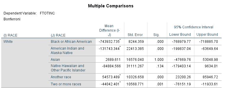
Now we see some points of interest. As you’d expect knowing what we know from prior research, race seems to have a pretty strong influence on a person’s income. (Notice I didn’t say “effect”—we don’t have enough information to establish causality!) The significance levels for the mean of White people’s incomes compared to the mean of several races are .000. Interestingly, for Asian people in the US, race appears to have no influence on their income compared to White people in the US. The significance level for Native Hawaiians and Pacific Islanders is also relatively high.
So what does this mean? We can say with some confidence that, overall, race seems to influence a person’s income. In our hypothetical data set, since we only have race and income, this is a great analysis to conduct. But do we think that’s the only thing that influences a person’s income? Probably not. To look at other factors if we have them, we can use a two-way ANOVA.
Two-way ANOVA and n-way ANOVA
A is a statistical procedure to compare the means of a variable across groups using multiple independent variables to distinguish among groups. For instance, we might want to examine income by both race and gender, in which case, we would use a two-way ANOVA. Fundamentally, the procedures and outputs for two-way ANOVA are almost identical to one-way ANOVA, just with more cross-group comparisons, so I am not going to run through an example in SPSS for you.
You may also see textbooks or scholarly articles refer to n-way ANOVAs. Essentially, just like you’ve seen throughout this book, the n can equal just about any number. However, going far beyond a two-way ANOVA increases your likelihood of a type I error, for the reasons discussed in the previous section.
A final note
You may notice that this book doesn’t get into multivariate analysis at all. Regression analysis, which you’ve no doubt seen in many academic articles you’ve read, is an incredibly complex topic. There are entire courses and textbooks on the multiple different types of regression analysis, and we did not think we could adequately cover regression analysis at this level. Don’t let that scare you away from learning about it—just understand that we don’t expect you to know about it at this point in your research learning.
Key Takeaways
- One-way ANOVA is a statistical procedure to compare the means of a variable across three or more categories of an independent variable. This analysis can help you understand whether there are meaningful differences in your sample based on different categories like race, geography, gender, or many others.
- Two-way ANOVA is almost identical to one-way ANOVA, except that you can compare the means of a variable across multiple independent variables.
Exercises
Think about the data you could collect or have collected for your research project. If you were to conduct a one-way ANOVA, consider:
- Which variable would be an appropriate dependent variable? Why?
- Which variable would be an interesting independent variable? Why?
- Would you want to conduct a two-way or n-way ANOVA? If so, what other independent variables would you use, and why?
Media Attributions
- Wasserstein, R. L., & Lazar, N. A. (2016). The ASA statement on p-values: context, process, and purpose. The American Statistician, 70, p. 129-133. ↵
- Steven Ruggles, Sarah Flood, Ronald Goeken, Josiah Grover, Erin Meyer, Jose Pacas and Matthew Sobek. IPUMS USA: Version 10.0 [dataset]. Minneapolis, MN: IPUMS, 2020. https://doi.org/10.18128/D010.V10.0 ↵
a group of statistical techniques that examines the relationship between two variables
"Assuming that the null hypothesis is true and the study is repeated an infinite number times by drawing random samples from the same populations(s), less than 5% of these results will be more extreme than the current result" (Cassidy et al., 2019, p. 233).
The characteristics we assume about our data, like that it is normally distributed, that makes it suitable for certain types of statistical tests
a statistical test to determine whether there is a significant relationship between two categorical variables
variables whose values are organized into mutually exclusive groups but whose numerical values cannot be used in mathematical operations.
a visual representation of across-tabulation of categorical variables to demonstrate all the possible occurrences of categories
a relationship between two variables in which their values change together.
when a relationship between two variables appears to be causal but can in fact be explained by influence of a third variable
a statistically derived value between -1 and 1 that tells us the magnitude and direction of the relationship between two variables
The strength of a correlation, determined by the absolute value of a correlation coefficient
Occurs when two variables move together in the same direction - as one increases, so does the other, or, as one decreases, so does the other
Occurs when two variables move together in the same direction - as one increases, so does the other, or, as one decreases, so does the other
occurs when two variables change in opposite directions - one goes up, the other goes down and vice versa
occurs when two variables change in opposite directions - one goes up, the other goes down and vice versa
A statistical method to examine how a dependent variable changes as the value of a categorical independent variable changes
a statistical procedure to compare the means of a variable across three or more groups
a statistical procedure to compare the means of a variable across groups using multiple independent variables to distinguish among groups
