12.1. Pre-experimental Designs: What You Should Not Do

Somewhat ironically, a good strategy for learning about experimental design is to start with designs that, for various reasons, just don’t meet the requirements we discussed earlier for concluding that a causal relationship exists between two variables. Technically, we call these approaches pre-experimental designs, because they have not yet achieved a “true” experimental design that is internally valid. We’ll follow a fictitious example of a social experiment as we go through some of the basic decisions about its design.

Using Pretests and Posttests to Measure the Effect of a Treatment

Let’s say a startup company created a fancy new educational app, AddUpDog, which teaches kids math. We want to know if regular use of the app actually improves math skills. For our social experiment assessing the app’s effectiveness, we decide that we’ll find a group of 50 fourth-graders (our research participants, or test subjects) and then have them each use the math app for 10 hours. Then we will give them a standardized math test and see how they score.

Let’s visualize what we’re doing. As we did in Chapter 3: The Role of Theory in Research with concept maps, it is helpful to create a design diagram for our experiment that lays out the key variables we’re working with. In the design diagram illustrated in Figure 12.1, our independent variable is the use of the AddUpDog math app, and our dependent variable is children’s scores on a standardized math test.

Even in the social sciences, scientists conducting experiments will call their independent variable the stimulus or treatment—language closely associated with lab experiments in the physical or medical sciences, where a specific intervention or factor is being observed within the lab setting. (The independent variable and dependent variable may also be referred to as the presumed cause and presumed effect, respectively—“presumed” because we do not yet have evidence that a change in our independent variable truly is the cause of any changes in our dependent variable.) In the study we’re designing here (depicted in Figure 12.1), our stimulus is having our participants spend 10 hours on the math app. This happens during “Time 1,” the start of the experiment. Then, during “Time 2” (say, a week after the participants use the app), we give them the math test.

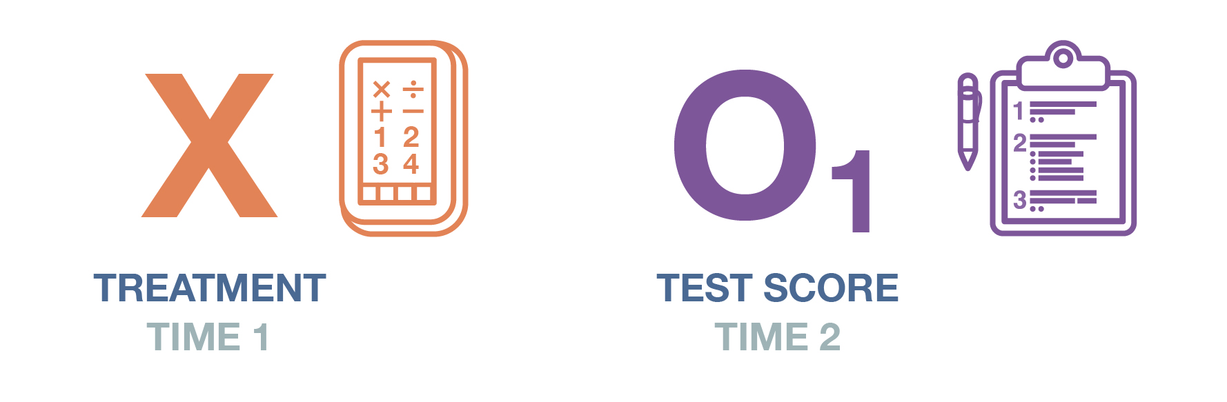
Let’s say all the children score high on the test after using the app for 10 hours. Specifically, their average score was 95 out of 100. We happen to know that the average score for fourth-graders on this test is 73 out of 100. Clearly, the app works, right? The kids used the app, took the test, and scored very high. Ergo, it is empirically proven that this app makes kids smarter. Time to slap on a Science™ endorsement on AddUpDog’s App Store description!

Not so fast. Has our experiment really given us strong evidence that AddUpDog improves test scores for fourth-graders? No, and that’s because our experiment is not internally valid. One obvious problem with our experiment’s design is that we don’t have a previous test score (before using the app) from this group to use for comparison. In experimental lingo, the previous test would be called a pretest. As shown in Figure 12.1, in this experiment we only have the posttest scores (the scores after the stimulus is introduced). As a result, we can’t really tell if the students improved or not. Yes, they scored high on our posttest, but it could be that we are experimenting on a class of fourth-graders who simply had very high math scores to begin with.

To address this problem, we decide to add a pretest (see Figure 12.2). Specifically, we give the kids the standardized math test during one given week (Time 1). We then have them do 10 hours on the app (Time 2). The following week (Time 3), we give them the same—or a similar—test to see if their scores have improved (we’ll talk later about why or why not we might not give them the exact same test). A change in their scores between those time periods—positive or negative—would give us some sense that using the app had an effect on the kids’ measured math skills.

Note, too, that by tracking the values of the dependent variable before and after, we establish temporal precedence, the second criterion for causality we discussed above. If the independent variable truly does have an impact on the dependent variable, introducing the stimulus will be followed by an increase in the value of the dependent variable sometime between the pretest and posttest. This outcome tells us something about the direction of any causal relationship that exists. If we had only cross-sectional observational data on students’ app usage and math scores, for instance, we might observe a strong correlation between the two variables, but we would not be able to say if the app was raising math scores, or if higher-scoring math students happened to use the app more. In other words, the use of this experimental design addresses problems of reverse causality (described in Chapter 3: The Role of Theory in Research)—when what we think is the independent variable is actually the dependent variable.

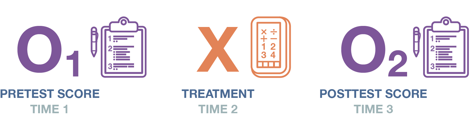
Our revised experiment has what we call a pretest-posttest design (or just pre-post design for short). With both tests in place, we can tell how much the students’ test scores changed after using the app between Time 1 and Time 3. Let’s say the average score jumped between the pretest and posttest—from 71 to 95. That’s a 14-point increase! Obviously, our math app is responsible. We should report our results to the Department of Education, maybe fire off an email to the Gates Foundation about getting an education innovation grant …

Hmmm, or might there still be other reasons that the kids’ scores went up?

Threats to Internal Validity When You Don’t Have Control Groups

Even with the revised experimental design we’ve just implemented, we remain unable to rule out many possible alternative explanations for the results we observed in our experiment. Here are some important additional factors we need to consider, which fall under the broad category of threats to internal validity:

1. History. The change we observed over time in our dependent variable might have been caused in whole or in part by an extraneous event—something that happened outside our lab setting but that nevertheless affected the results we measured in the lab. We call this the history threat to internal validity (or history effect). This might indeed be a “historical” event, such as an event that affected all of society at the same time (say, a terrorist attack during the time period when we’re doing an experiment relating to people’s views on national security), but the term “history” here really refers to any event outside of the parameters of the experiment that nonetheless may be influencing our results—for example, a class that our participants also happen to be taking at the same time they’re being studied. The important thing is that the outside event in question occurred sometime between our pretest and posttest, which means we may mistake the impact of that extraneous event for the impact of our experimental treatment. In our math app example, it is possible that in the time between our pretest and posttest, some of the students could have watched an educational television program that was the true cause of their increased scores. Or the students may have had a refreshing recess break right before their posttest (but not before the pretest), meaning they were better able to focus on their second go.
2. Maturation. Especially during a long-running study, we need to account for the possibility that any changes we observe in the dependent variable between tests may have been caused by natural changes in our participants (a maturation threat or maturation effect) rather than by the experimental treatment per se. Say we are conducting an evaluation to see if a preschool program helps improve academic achievement later in childhood. The program—and therefore our evaluation of it—lasts for several years. By the time we conduct a posttest, the participants have become older. They have experienced general improvements in their intellectual ability that go beyond the impact of that one program (if it had an impact to begin with). Much like we saw with the history effect, lots of things may be going on simultaneously during the course of a long-term study like this one. Unless we could account for them, we would not want to chalk up any improvements in the children’s cognitive abilities just to the influence of the preschool program.
3. Testing. The testing threat to internal validity (or testing effect) involves concerns that giving our test subjects the pretest could itself have influenced their posttest scores. In our example, just showing the fourth-graders our math test would make them more familiar with the test format and content, meaning they are likely to score higher on the posttest than they otherwise would have. This bias toward improved scores on any evaluation done multiple times is rather obvious: after all, this is why test preparation companies make millions of dollars getting students to take pricey courses or buy practice materials to give them an edge on the SAT, ACT, GRE, and other standardized tests.
4. Instrumentation. In our math app example, suppose we decide we don’t want to give our fourth-graders the exact same math test as a posttest, given that their scores may increase because of the testing effect (that is, because they are familiar with the test from the first time they took it.) We change the questions on the posttest so that they’re equally hard but not exactly the same. The problem, of course, is that we need to be sure our posttest actually is equally hard, so that any changes in students’ scores can’t be attributed to the changed nature of the test. This latter problem we’re dealing with is called an instrumentation threat (or instrumentation effect)—the possibility that the difference between our pretest and posttest scores isn’t due to the experimental stimulus or treatment, but rather to changes in the administered test (our study’s “instrument”). If the posttest we give our fourth-graders has a lower degree of difficulty than the pretest, this instrumentation issue will give them, on average, higher posttest scores. In turn, we may conclude, erroneously, that the app had an effect. Conversely, if the pretest is easier than the posttest, the kids will have lower scores on the posttest, and our experimental results may understate the effectiveness of the app. The instrumentation threat also applies more broadly to cases where the kind of testing we do itself shapes our results to an extent that we may mistake that effect for the influence of the independent variable.
5. Regression to the mean: Another possible explanation for our findings is a phenomenon called regression to the mean (also called just regression, though note that this is different from another type of “regression” we’ll talk about in Chapter 14: Quantitative Data Analysis, which has to do with using statistics to measure the relationship between two variables). Regression to the mean refers to a statistical tendency that may make us observe changes in the dependent variable across the pretest and posttest that don’t have to do with the influence of the independent variable. Specifically, we may have a situation where a group’s performance on the pretest happens to be particularly extreme, and their later results on that measure move toward what we typically expect—the mean—simply because the second test, the posttest, didn’t happen to have such extreme cases. Let’s say some of our fourth-graders using the math app are having a bad day and happen to score very low on our pretest. By statistical theory, they are likely to score higher on the posttest (closer to the mean or average). Therefore, their improved scores in this case will be due to regression to the mean, rather than to the influence of the math app. (Note that the exact opposite could also be true—the students happen to score high on the pretest, and then, because of regression, they score lower on the posttest.) Regression to the mean is often a problem when there is a cutoff for admission into an experiment. Say we only pick students for our study who score low on their math scores because we want to see whether the app is effective for struggling students. Because of this research design, however, we should expect some regression to the mean—that is, the results of the posttest to be generally higher. Some of the students selected for our study just had exceptionally bad luck on that first test, and their scores on subsequent tests will be closer to their average performance.

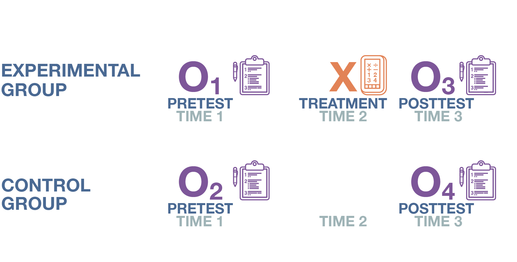
So how do we account for all these possible alternative explanations in our experiment? The standard scientific approach is to add a control group. A control group is a sample of participants who do not receive the experimental stimulus. Nevertheless, we include them in our study and measure their scores on the dependent variable.

What does having a control group give us? As illustrated in Figure 12.3, the control group’s outcomes can be compared to those of the experimental group (also known as the treatment group), which is composed of the participants who do receive the stimulus or treatment. Setting up the experiment in this way helps rule out the threats to internal validity we’ve just described. Both the control group and treatment group should be subject to the history, testing, regression, etc., effects, meaning we still should be able to measure the effect of the stimulus, which only the experimental group received.

Threats to Internal Validity When You Don’t Have Randomization

Let’s say that the average posttest score for our experimental group—the children who used the math app for 10 hours—does turn out to be higher than the average score for our control group who didn’t use it. Can we finally conclude that the math app is effective?

Not yet, unfortunately. It’s possible that the differences we observed between the control and experimental groups existed before we administered the stimulus to the experimental group. As a result, we may falsely believe that the independent variable explains the two group’s divergent scores when preexisting differences really do. In our example, the fourth-graders in our experimental group may have been better at math than the control group students were even before they started using the math app. This is what we call a selection threat (also known as a selection effect). In this scenario, a certain kind of participant is more likely to be selected for the experimental group, and as a result, the two groups diverge from one another on the outcome being measured in ways that have nothing to do with the stimulus given to the experimental group.

For instance, let’s say that when we were looking for kids to test our AddUpDog app, we sent out a form to fourth-grade classes asking for volunteers. We asked the students’ parents if they were willing to have their child participate in the study for $20, and we gave them the option to be in the experimental group or control group. Many parents might have chosen the control group for their child because they wanted the money but they didn’t want to sit their kid down to use an educational app for 10 hours. Let’s say that this was especially the case for the parents of kids who were already not doing well in math class. Then our control group might perform more poorly than the experimental group on our math test regardless of whether the app works. Students who struggle at math were just more likely to be selected for the control group to begin with. The differences between our two groups created bias—specifically, selection bias—in our results.

You might be wondering here why the pretest doesn’t help us avoid this problem of selection. The answer is that it does: if we do a pretest, and the experimental and control groups are different on key variables, we clearly have a problem. But what do we do then? Even with the pretest alerting us to the fact that our comparison groups are not alike, we’re still stuck with our selection problem. In our math app example, let’s say we decide to have one fourth-grade class serve as our experimental group, and another fourth-grade class serve as our control group. Then, through our pretest, we discover that the students in one of these classes happen to be math geniuses. At this point, do we really need to recruit an entirely new sample of participants? Maybe, but luckily we can avoid this problem altogether if we set up our experiment with randomized control and treatment groups, as we will describe in the next section.

Selection bias is a major problem in the social sciences, and it occurs more frequently than we might expect. For instance, in the Stanford prison experiment we discussed in Chapter 8: Ethics, one of the criticisms of the study’s research design (beyond all the ethical problems we discussed earlier) was that the men who actually volunteered for the study were a special, self-selected group. The newspaper advertisement that recruited the study’s participants mentioned that the researchers were conducting a “psychological study of prison life.” A study by Thomas Carnahan and Sam McFarland (2007) used almost the exact same text for a newspaper ad recruiting study participants, except sometimes they excluded mention of “prison life” (thereby creating a control group in Carnahan and McFarland’s experiment). They found that those who responded to the ad with the text “prison life” scored higher on measures of aggressiveness, authoritarianism, Machiavellianism, narcissism, and social dominance and lower on measures of empathy and altruism than responders to the ad that didn’t mention “prison life.” In other words, the people who responded to the Stanford prison experiment’s ad may have been more sadistic to begin with, which may suggest that the guards’ abusive behaviors during the course of that study may have been due at least in part to that selection bias rather than the prison scenario itself, as the original study claimed.

Another issue related to the study sample is attrition bias. This refers to the possibility that certain types of participants may be more likely to drop out of our study. If the experimental and control groups are different in terms of who drops out of each, that difference may actually be responsible for our study’s results, rather than the influence of the independent variable itself. (Sometimes this bias is called mortality bias, given how test subjects in a classic scientific lab experiment would die out or otherwise leave the study.) In our app example, if for some reason low-performing students disproportionately drop out of the experimental group (perhaps because the app bores them and they don’t want to do the full 10 hours of screen time), we would end up only with high-performing students in that group. This could produce a higher posttest average in the experimental group than in the control group. The key problem here is not so much that people dropped out, but that (1) they dropped out to a different extent across the two groups, and (2) those who dropped out had disproportionately high or low scores on the dependent variable. (We’ll return to this issue of attrition bias and its close cousin, nonresponse bias, in Chapter 13: Surveys.)

So how do we actually address the threats to internal validity posed by selection bias and attrition bias? We’ll want to find a way to make sure that the experimental and control groups in our study start out as similar as possible on the variables that matter. And we’ll want to make sure they remain that way, and that a disproportionate number of dropouts in one group is not skewing our observed outcomes. Randomly assigning participants to these two groups is the most straightforward way to address selection bias, as we will discuss in the next section. As for attrition bias, experimenters will go to great pains to ensure that members in both groups stay in the study, but there is often no easy solution to this problem when it crops up.