7.2. Deciding on the Correct Level of Measurement

When social scientists measure concepts, they often use the language of variables and attributes. In this context, you can think of a variable as a grouping of two or more characteristics, and attributes as the characteristics that represent values or categories of a variable. For example, the variable “dog breed” would contain attributes like terrier, retriever, and shepherd. How many attributes a variable has, and how those attributes can be distinguished from one another, are especially important in quantitative research. A variable’s attributes determine its level of measurement, which in turn tells us what kinds of mathematical operations can be applied to the variable when conducting a quantitative analysis.

For practical purposes, the three possible levels of measurement in sociology are nominal, ordinal, and scale. (See the sidebar Deeper Dive: Interval and Ratio Levels of Measurement to learn about even more granular levels of measurement.) A variable at the nominal level has attributes that are different from one another, but unlike for the other levels of measurement, those attributes do not follow any mathematical order.

Dog breed is a good example of a nominal-level variable. In 2022, the American Kennel Club (AKC) recognized 199 dog breeds. Each breed’s ideal physical traits, movement, and temperament are carefully described in a “breed standard,” which specifies its unique characteristics. Figure 7.2 provides an example of two dog breeds whose characteristics are different from one another.

To identify a nominal-level variable, ask yourself one question: “Can I rank the variable’s attributes in order from high to low (or low to high)?” The ranking has to make logical sense. For example, a higher-ranked attribute must be higher in some characteristic than the ones below it, such as a higher frequency of occurrence, higher amount of time spent, higher level of ability, or higher degree of satisfaction. If your answer to this key question is “No”—the variable’s attributes cannot be ranked—then the variable is nominal level. If your answer is “Yes,” then the variable should be measured at a higher level.

The answer to this question for our “dog breed” variable is clearly “No”: the diverse categories of dogs captured by the variable do not have any inherent ordering to them. That said, two conditions must hold for this nominal-level variable—or, for that matter, any variable we want to analyze quantitatively. First, its attributes must be mutually exclusive: the categories must all be different from one another, with no overlaps. Second, its attributes must be collectively exhaustive: the categories should cover all the conceivable instances that might occur—that is, they should “exhaust” all possibilities. (Sometimes these two conditions are abbreviated as MECE, or “mee-cee”: mutually exclusive + collectively exhaustive.)

How do you ensure that your nominal-level variable is exhaustive? An easy way to do so on surveys is to allow respondents to answer “none of the above” or “other” in answer to the question. That way, the survey question’s response categories—the answers available for each question—will truly cover all possibilities (we’ll have more to say about survey question design in Chapter 13: Surveys). To make our dog breed variable exhaustive, we could create two “other” categories: an “other breed” attribute to cover dogs who are purebred, but not of a type recognized by the AKC, and a “mutt” attribute to cover dogs of mixed or unknown breeds.

It can be trickier at times to ensure that your variable’s attributes are mutually exclusive. In plenty of situations, “overlaps” across categories are important. For instance, if you are measuring race, you’d want to account for the large number of people with mixed-race identities. Creating an “other” category is the simplest way of addressing this issue, but you may also want to create separate categories for common multiple-race identities. (You can also create multiple variables to preserve information about cases that straddle multiple categories, as we discuss in Chapter 14: Quantitative Data Analysis.)

Following are some examples of nominal-level variables that are commonly used in sociological research. Each of these variables has a range of attributes that are mutually exclusive and collectively exhaustive.

Table 7.1. Sociological Examples of a Nominal Level of Measurement

In Table 7.1, we’ve numbered the responses—something you will want to do whenever you input survey data into a quantitative dataset.^[1] Note that although the attributes in this table are numbered, the order of the attributes for nominal-level variables is always arbitrary. Protestants, for example, could have been numbered as 1, 2, 4, 5, 103, or any other unique number. (Sometimes surveys take advantage of their flexibility to number response categories by grouping together similar categories in a number range—for instance, making Catholics 10, but putting Protestant denominations in the thirties, such as 31 for Lutherans, 32 for Methodists, and so on.)

After nominal-level variables, the next higher level of measurement is the ordinal level. Like nominal-level variables, ordinal-level variables must have attributes that are mutually exclusive and collectively exhaustive. Unlike nominal-level variables, they have attributes that can be ranked from high to low (or from low to high) using some kind of meaningful comparison. For example, we could ask survey respondents to rate how healthy they feel from “poor” to “excellent.” We would then have an ordinal-level measure of perceived health.

Ordinal-level variables are very common in quantitative sociological research. In the surveys you’ve taken, you’ve probably come across Likert scales, which are used to measure the intensity of people’s opinions. (By the way, it’s pronounced LICK-ert—something that many professional sociologists get wrong!) To measure agreement with a particular statement, Likert scales will often use four or five ranked response categories that range from “Strongly agree” to “Strongly disagree.” Consider this question asked in the General Social Survey, a survey of the attitudes of U.S. adults taken every two years:

How much do you agree or disagree with the following statements? American culture is generally undermined by immigrants.

1. Strongly agree

2. Agree

3. Neither agree nor disagree

4. Disagree

5. Strongly disagree

In this example, “strongly agree” (numbered as 1) represents the most positive attitude toward the statement, while “strongly disagree” (5) represents the most negative attitude toward the statement. “Neither agree nor disagree” (3) is an intermediate category, representing a neutral or undecided attitude.

The only thing that matters when we number ordinal-level variables is the ranking, not the specific number assigned. For instance, we could easily switch 1 to mean “strongly disagree” and 5 to mean “strongly agree.” Under this new numbering, increasing values would mean greater agreement with the statement; in the original, they mean greater disagreement. Also, the response categories do not have to be numbered from 1 to 5—we could number them 0 to 4, or −2 to +2, for instance. For ordinal-level variables, the numbering could be reversed or be different numbers entirely, as long as the numbers are still ordered in relation to each other.^[2]

Ordinal-level variables differ from higher-level variables in one key way: although we can rank the attributes of ordinal-level variables, we cannot determine the exact distance between those ranks. Figure 7.3 visualizes what we mean by “distance” using the example we previously mentioned: level of perceived health.

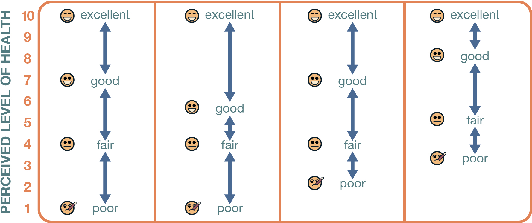
For our variable of each respondent’s perceived level of health, the attributes are excellent, good, fair, and poor. Let’s assume we actually know how healthy each person is on a scale of 1 to 10 scale, with 10 being the healthiest (for various reasons, this is simplistic, but let’s go with it!). How do the response categories for our ordinal-level variable of perceived health map onto that scale? We know that “excellent” represents the highest level of health and “poor” the lowest, but we do not know where other responses would put us on our “real” 1⁠–10 scale—is a response of “good” a 6, 7, or 8? It’s possible that each respondent interprets words like “good” or “fair” in different ways. One person may think of “good” as the equivalent of 8 on the 1⁠–10 scale, whereas another person thinks of it as a 6. Likewise, we know that “good” means worse health than “excellent,” and “fair” means better health than “poor,” but we don’t know that whether the distance between one particular category and another is 1, 3, 5, or 7 points—or whether those categories would be spaced out equally across such a scale. All we know is the rank ordering.

Table 7.2 provides more examples of common ordinal-level variables in sociology. As you review these examples, think about the distances between the response categories and whether they do, or do not, change as you move across the continuum. Also think about what the numbering means—for example, as the numbers rise, what exactly is increasing?

Table 7.2. Sociological Examples of an Ordinal Level of Measurement

You might have noticed that two of the variables in this table—frequency of religious service attendance and family income—could, in theory, be measured more precisely. It’s often difficult, however, to obtain precise and accurate values for these variables. Do people remember how much money they made in dollars before taxes last year, or exactly how many times they went to religious services last year? Maybe some do, but many others will be stumped. Particularly for income, people may feel uncomfortable giving you a specific number. Such sensitive or difficult-to-recall variables are often collapsed into ordinal groups, so that we can tell whether one person has a higher level than another, but not exactly how much higher.

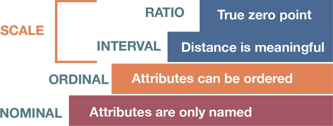
To summarize what we’ve discussed so far, nominal-level variables must have attributes that are mutually exclusive (no overlaps) and collectively exhaustive (all possible responses accounted for). Ordinal-level variables add another condition: rank ordering (the attributes correspond to higher or lower ranks). The next-highest level, the scale level, meets these three conditions and adds one more: equal intervals. You can see the relationships among these three levels of measurement visualized in the hierarchy shown in Figure 7.4, which goes from the variables with the least to those with the most conditions.

When we say that a scale-level variable has “equal intervals,” we mean that the distance between each pair of adjacent ranks or points on the scale is equivalent. Social scientists often use the term continuous variable interchangeably with “scale-level variable,” and you might want to think of the values of a scale-level variable as lying on a continuum much like a number line. Every point along that continuum has a possible value, and the distances between the adjacent ranks—on a number line, the numbers next to each other—are equal.

Perhaps the scale-level measure that you come across most often in your daily life is temperature. Both the Fahrenheit and Celsius scales meet this additional condition of equal distances on their scales measured in degrees: the difference between, say, 20 and 21 degrees is the same as the distance between 42 and 43 degrees. With an ordinal-level measure of temperature—say, “hot,” “lukewarm,” and “cold”—we wouldn’t know if the distance between “hot” and “lukewarm” was equivalent to that between “lukewarm” and “cold.” With scale-level variables, we know the distances, and they are equal across each rank (in this case, each degree of temperature).

Table 7.3 presents sociological examples of scale-level variables—which would include all the variables that we have not already categorized as nominal or ordinal level.

Table 7.3. Sociological Examples of a Scale Level of Measurement

Whether the distance between a variable’s attributes is measurable and equal is critical because it affects the specific procedures we use to analyze the data. As we will discuss further in Chapter 14: Quantitative Data Analysis, we can do certain calculations—such as determining means and medians—for scale-level variables that we can’t do for nominal-level and ordinal-level variables. (Variables at those lower levels of measurement are referred to as categorical variables to distinguish them from continuous variables.)

If you have the choice, it’s generally best to collect data at as high a level of measurement as possible. That’s because higher-level data can be grouped and converted into a lower level of measurement. For example, if we collect scale-level variables like an adult respondent’s age at a lower level—say, in ordinal groups of 18 to 34, 35 to 49, 50 to 64, and 65 and older—we can never recover the precise ages during data analysis. If the only thing you know is that a person is in the age range of 18 to 34, it is impossible to say exactly how old they are. It could be 18, or 34, or anything in between. You would also run into problems taking the halfway mark—say, 26—to stand in for all the people who chose that response, because it may be that most of the people who answered that way fell in the lower (or upper) range of that category.

Conversely, if you know your respondents’ specific ages, you can easily convert your data into ordinal groups at any point in your analysis. That said, researchers often choose not to measure some concepts at the scale level even when they can do so. As we alluded to earlier, getting respondents to recall precise figures can be difficult, and they are especially reluctant to be pinned down on specifics in regards to sensitive topics like money, sex, or drug use.

Deeper Dive: Interval and Ratio Levels of Measurement

Scientists further divide scale-level variables into interval-level measures and ratio-level measures. The critical distinction between these two levels of measurement is that ratio-level variables have a true zero point. Having a “true zero point” means that zero on whatever scale is being used refers to the complete absence of the phenomenon being measured. Let’s take the example we used previously, temperature, which measures thermal energy.

For a measure of temperature to have a true zero point, a zero on the scale should refer to an environment that has utterly no thermal energy. That does not hold for the Fahrenheit or the Celsius scales. Indeed, both scales can go below zero into negative numbers (although you might prefer a wintry day with temperatures below zero in Fahrenheit to one spent below zero in Celsius). Because they do not have a true zero point, the Fahrenheit and Celsius scales are measured on the interval level.

This distinction has mathematical importance. The fact that Fahrenheit and Celsius do not have a true zero point means that any ratios of their numbers are not meaningful. For example, on both scales, a room heated at 40 degrees is not twice as hot as one heated at 20 degrees (2:1 ratio); there is not twice as much thermal energy in the first room as there is in the second. Likewise, a substance cooled down to −30 degrees is not three times as cold as one cooled to -10 degrees (3:1 ratio). To be able to say that such ratios are meaningful, we need the measure to have a zero point that actually refers to nothing—that is, the complete absence of whatever we’re measuring. For temperature, it’s the point at which there is zero thermal energy in a system—the coldest temperature possible.

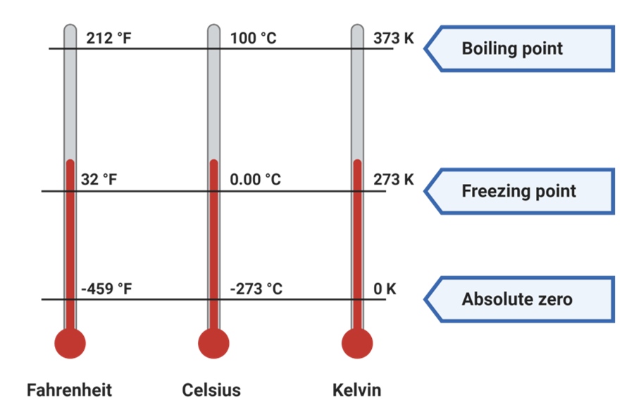
As you might remember from other classes, this is actually true on the Kelvin temperature scale. (As you can see in Figure 7.5, Kelvin is simply Celsius adjusted upward by 273 degrees, with 273 Kelvin equivalent to 0 degrees Celsius.) Zero Kelvin is the complete absence of thermal energy. This means that the Kelvin temperature scale has a true zero point, and it is measured on the ratio level—the highest level of measurement.

For such variables, ratios are meaningful. Twenty degrees on the Kelvin scale is twice as hot (has twice as much thermal energy) as 10 degrees. A person who is 12 years old is six times as old as a 2-year-old. $100,000 in cash is 10 times as much as $10,000. A 20-year-old who has lived in the United States all her life has lived there four times as long as someone who moved to this country five years ago. For all these variables, the zero on the scale has a meaning, even if it is a social or cultural meaning. For example, the zero point for age is the point right before birth, the point of “zero” age (it’s worth noting that some cultures have historically tacked on nine months to that age to account for time in the womb). Zero is also meaningful for a variable measuring the number of years you have spent at your current address—although whether that point of measurement begins right when you walk over the threshold of your new home or when you sign an official document is often arbitrary.

When you are doing quantitative data analysis in sociology, interval and ratio levels don’t actually have any practical differences. You can use the same analysis techniques with each. In the research literature, you’ll often see them both referred to as scale-level variables. When you see this term, keep in mind that this is not an additional level of measurement. Instead, it refers to both interval and ratio levels.