12.2. Randomized Controlled Designs: What You Should Do

What we call a “true” or classical experimental design is the gold standard for conducting experiments, a strategy that maximizes the internal validity of our study. As illustrated in Figure 12.4, a classical experimental design has all the features we’ve described above: a stimulus or treatment, an experimental and control group, and a pretest and posttest (though, as we’ll discuss later, sometimes experimenters for various reasons choose not to conduct a pretest). But we need to go one step further to avoid the selection effect—the danger that our experimental and control group may start off differently on the key outcome measure we’re interested in, thereby leading us to false conclusions about the effect of our treatment on the outcome measure. Specifically, we will want to assign participants into our two groups by using a simple statistical technique that increases the likelihood that the experimental and control groups will be similar: randomization.

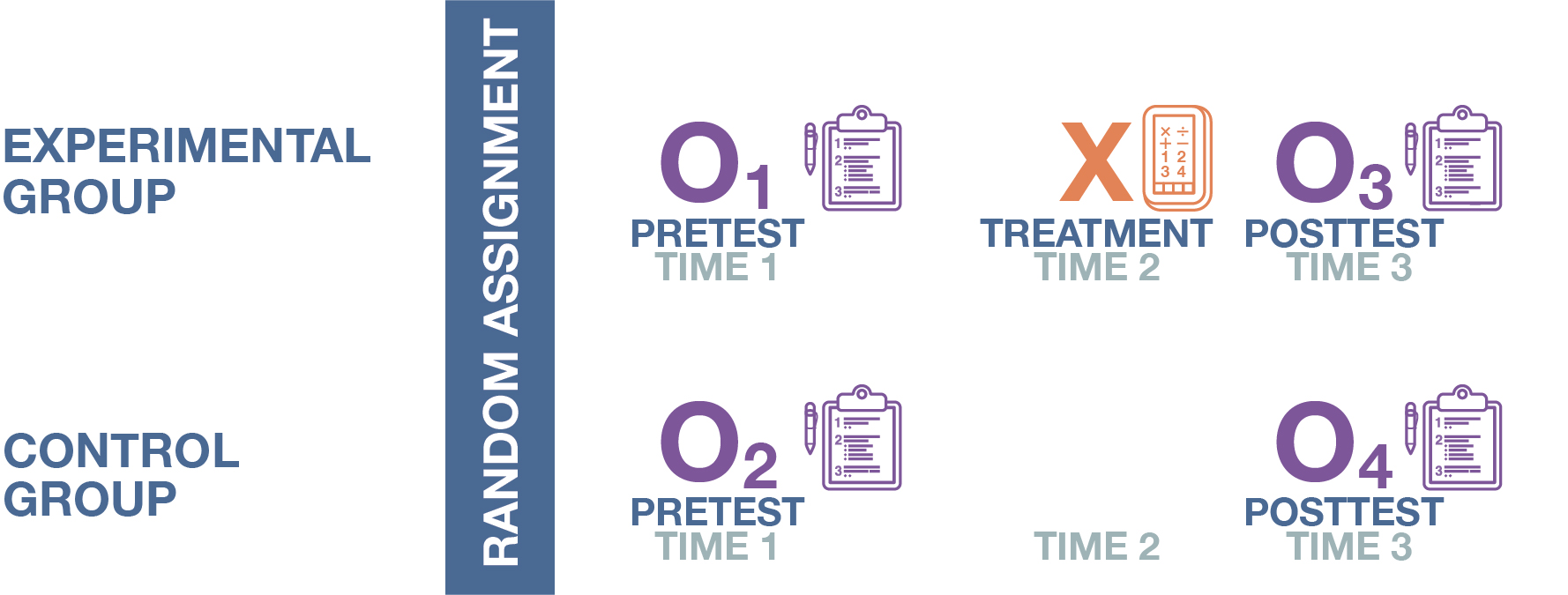
Random selection is an important component of probability sampling (described in Chapter 6: Sampling). As you might remember, one method of making sure that your sample is truly representative of the population of interest is to gather a random sample—say, assigning a number to each member of the target population and then using a random number generator to choose your sample’s cases from that enumerated list. In experimental design, the use of randomization is a bit different. Instead of selecting cases at random from a larger population, random assignment within an experiment means that we assign each of the study’s participants to either the experimental and control groups at random—that is, with an equal 50 percent chance to be assigned to either group. As illustrated in Figure 12.4, if two students agree to participate in our math app experiment, we could flip a coin to assign the first student to the experimental group (heads) or the control group (tails), with the second student automatically assigned to the other group. We can continue doing this until we have a sufficient number of people in the two groups. (In practice, real researchers typically just use computer programs to assign their participants instantly to either group.)

What’s the point of all this? Using randomization means that there is unlikely to be any substantial differences between the experimental and control groups at the outset of the experiment. By “any substantial differences,” we mean that the two groups will obviously not be exactly the same on all characteristics, but they will usually be quite similar. After we randomly assign fourth-graders to the experimental and control groups in our math app example, the average math scores for the two groups are likely to be close on any pretest we give them. In fact, the two groups are likely to have similar characteristics on any measure—a similar proportion of brown-eyed participants, similar preferences for K-pop music, similar enthusiasm for pickleball—given that we placed everyone at random in our two groups. On occasion, we may come across extreme cases of participants who skew the measures for our otherwise neatly comparable experimental and control groups, but so long as we are faithfully using random assignment, the average characteristics should be more or less the same across the two groups.

What’s more, simple statistical theory tells us that the larger the participant pool we’re drawing upon for our experimental and control groups, the less likely there are to be any meaningful divergences between the two groups. For example, if we’re gathering participants for our AddUpDog evaluation from a pool of just 10 fourth-graders (therefore assigning five participants to each group), our randomized selection process may very well wind up stacking four or five math geniuses in one of our groups. Yet once we reach a pool of, say, 100 students (50 participants in the experimental and control groups), the magic of randomization will have muted any differences in math ability between the two groups, making us confident that we can compare their outcomes in an apples-to-apples manner after we administer the AddUpDog treatment.

It may be helpful now to review the various benefits of a true experimental design for causal inference (again, our ability to conclude that a change in our independent variable truly causes a change in the dependent variable.) By manipulating the independent variable and keeping all other factors constant within the lab setting, we are able to rule out any confounders that may independently influence the dependent variable. If we just examined the correlation between two variables using observational data, it would be quite easy to be tricked by spurious correlations, but through the use of control groups and random assignment we have accounted for all alternative explanations for the outcomes we see. For this reason, drug trials and other clinical studies that use this classical structure are called randomized controlled trials (RCTs)—“randomized” referring to random assignment, and “controlled” to the use of treatment and control groups. Other variants of the term are randomized controlled experiments or randomized controlled studies.

With this set of safeguards in place, a classical experimental design allows us to conclude with confidence that we have measured the impact of the independent variable “all other things being equal” (a condition known by the Latin term ceteris paribus). This is a basic condition for being able to make a causal argument that any treatment is driving changes in the dependent variable, because it means we have ruled out any competing causal stories. And to repeat, random assignment across the experimental and control groups helps ensure this condition, because it makes the two groups comparable on all characteristics. In fact, with randomization, we can say the control group is a reasonable representation of our counterfactual: what would have happened to the experimental group if the treatment had not actually occurred. The counterfactual is like the science fiction notion of an alternate reality—had we gone back in time and chosen not to give the stimulus, what would we have seen? This is something that we never really know with observational data, but with a proper experimental design, the control group is an apt stand-in for our counterfactual.

Interpreting the Results of a Randomized Controlled Experiment

Now that we’ve randomly assigned our participants into the two groups, how do we interpret the results of our posttest? Picking up our example again, there are several things we want to look at in order to make a rigorous case that the AddUpDog app actually has—or does not have—an effect on students’ math scores. First, the average math scores for the experimental and control groups on the pretest should be similar. Since the two groups were randomly assigned, this should not be a problem, as we’ve just discussed. Nevertheless, comparing the groups in this way is often worth doing, because it may very well be the case that their pretest scores are very different—perhaps we did something wrong in the randomization process, or perhaps we were just unlucky. If the two groups do diverge substantially, we may need to recruit more participants or pursue other means (beyond the scope of this textbook) to address this issue.

Once we’re confident in the similarity of our experimental and control groups, we can proceed with our analysis by seeing if three distinct patterns appear in our results. These patterns need to hold in order for us to conclude that the relationship between the independent and dependent variables we’re observing is truly causal. The three conditions are captured by the three questions listed below. Note that all three questions assume we are testing whether the stimulus or treatment increases scores on our outcome measure. In the AddUpDog example, for instance, we’re evaluating whether using the app raises kids’ math scores. The questions should be reversed (e.g., “higher” swapped out for “lower”) if we are testing whether the stimulus or treatment actually reduces measured levels of the dependent variable.

Condition 1: Within-group pre-to-posttest change. Is the experimental group’s posttest score higher than its pretest score? If the treatment (here, math app usage) truly has an effect on the dependent variable (here, math test scores), then the posttest average for the experimental group should be higher than its pretest average.

Condition 2: Between-group posttest difference. Is the experimental group’s posttest score higher than the control group’s posttest score? If the treatment truly has an effect on the dependent variable, then the experimental group’s posttest average should be higher than the control group’s posttest average.

Condition 3: Between-group differences in pre-to-posttest change. If the control group experienced an increase in its average score between the pretest and posttest, is that increase smaller than any increase experienced by the experimental group between its pretest and posttest? Note that this condition is relevant only when the control group’s scores increase in its scores between the pretest and posttest. And observing that increase by itself does not rule out a causal relationship between the independent and dependent variable. After all, it’s possible that the various alternative factors we mentioned earlier (e.g., testing effects) are at work here, too, which may mean that everyone’s scores—those for the experimental group and the control group—go up between the pretest and posttest. That said, if the control group experiences such an increase between the pretest and posttest, that increase should be smaller than the increase experienced by the experimental group.

If the answer to any of these questions is “no,” then our results indicate that there is no cause-effect relationship between the independent variable and dependent variable. The stimulus does not by itself cause a change in the dependent variable. But if the first two conditions hold (and the third one as well, if it is applicable), then we can conclude that the causal relationship exists—in our math app example, that the AddUpDog app truly does improve math skills. In fact, we can quantify the size of that effect by calculating the average treatment effect—the change in the dependent variable that we expect, on average, after the stimulus or treatment is received. The average treatment effect (sometimes abbreviated ATE) in a classical experimental design would be the difference between the experimental and control groups’ average scores on the posttest.

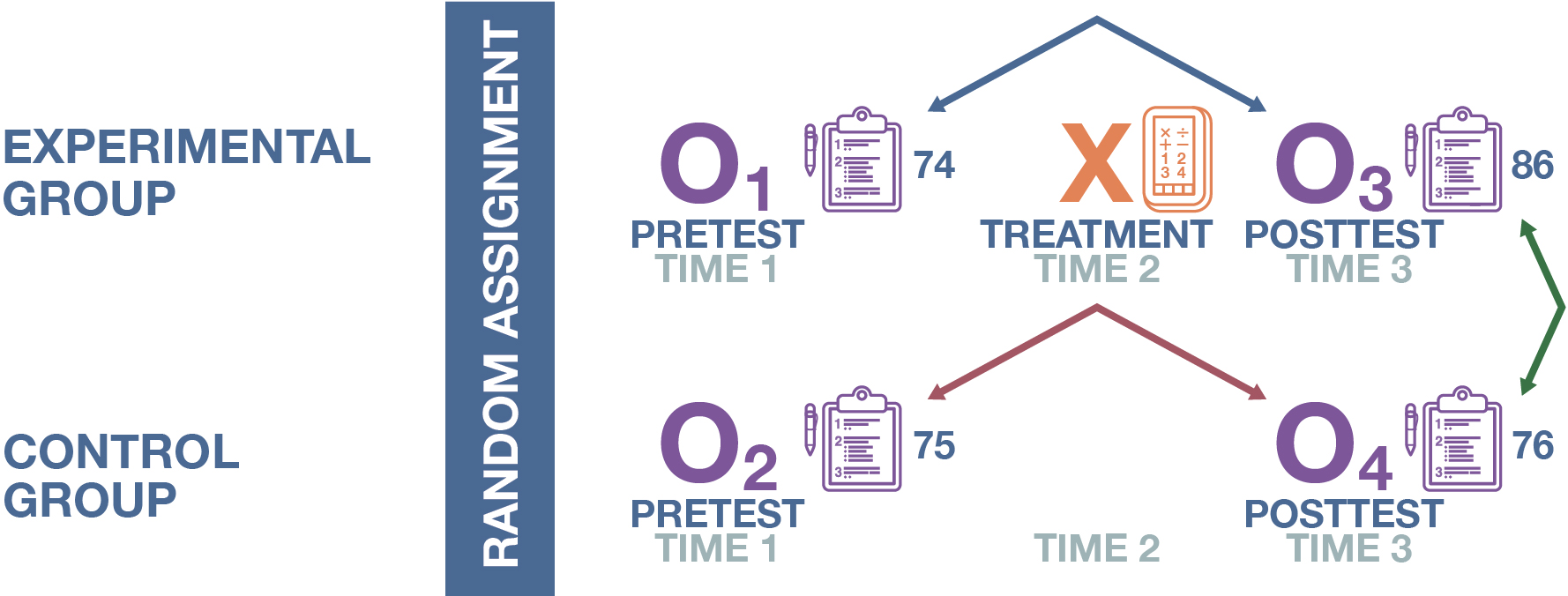
In Figure 12.5, we can see what the results of our AddUpDog experiment might actually look like. The numbers in the diagram refer to each group’s average on the math test (pretest or posttest) out of 100 possible points. As you can see, the pretests we conducted gave us a similar baseline for the experimental and control groups—74 and 75, respectively. Between the pretest and posttest, the experimental group’s math score rose from 74 to 86—satisfying Condition 1 above that the experimental group’s posttest must be higher than its pretest. And in line with Condition 2, we see that the experimental group’s posttest average of 86 is higher than the control group’s posttest average, which is 76. Finally, the control group’s math score rose slightly over the course of the experiment—from 75 to 76—meaning that Condition 3 is also relevant. When comparing scores for the two groups between the pretest and posttest, we see that the control group’s 1-point increase is smaller than the 12-point increase experienced by the experimental group across the same tests, satisfying Condition 3. All three conditions hold, and therefore we have evidence to believe that 10 hours of using our math app does lead to improvements in the math skills of fourth graders. (Note the very specific way we’re phrasing our findings here, which we will talk about more later in regards to the external validity of our experimental results.) Furthermore, we conclude that the average treatment effect here is 10 points—using the app, on average, boosts math scores by 10 points.