12.5. Quasi-experiments: Approximating True Experiments with Observational Data

When true experiments are not possible, researchers often use quasi-experimental designs. These studies are similar to true experiments, but they lack random assignment to experimental and control groups. As a result, they are vulnerable to many of the threats to internal validity we talked about—selection bias above all.

As we discussed earlier, social scientists who pursue field experiments often make do without random assignment or other features of a classical experimental design because the real-world setting doesn’t afford them that degree of control. They may tolerate a quasi-experimental approach because they explicitly want to generate findings with higher external validity. Beyond that specific consideration, however, quasi-experimental designs often make a lot of sense for researchers.

For one thing, controlled experiments are very demanding. Because participants are subjected to an experimental manipulation of some kind, experiments (whether conducted in a laboratory or in the field) require more of participants and are more intrusive in their lives than other research designs. As we discussed in Chapter 8: Ethics, the rules and guidelines that govern research today largely emerged in response to wildly unethical and dangerous experiments, including social scientific experiments. Sociologists who employ this methodological approach must be especially careful about following ethical principles to prevent abuses. These considerations figure not just into the informed consent process for recruiting participants, but also in the randomization process of assigning them to experimental and control groups—for instance, offering benefits based on a lottery, as with the Moving to Opportunity study, can be problematic depending on the type of assistance being offered. Many times, too, the decision about whether to use a classical experimental design is just not up to us. We may lack the resources of time or money needed to go that route, or we may not have the institutional support we need to structure our experiment in the most ideal way.

In this section we’ll talk about various quasi-experimental approaches that researchers may pursue for ethical or pragmatic reasons. When we can’t randomly assign subjects into control and experimental groups, the next best thing for us to do is to approximate that random assignment. There are two popular strategies for doing this. First, we can assign treatment and control groups ourselves, using a wide range of techniques like the ones we discuss below—from comparison groups and matching, to time-series and regression discontinuity designs. These quasi-experiments are much the same as all the other experiments we’ve been talking about so far, in that they are interventional experiments—that is, the researchers intervene in the experimental setting (here, to create the control and treatment groups). This approach can be contrasted with natural experiments. In this second kind of quasi-experiment, we creatively exploit events in the real world that serendipitously assign our participants to treatment and control groups for us. We describe this category of quasi-experiments in its own section below. Note that some techniques used in interventional quasi-experiments, such as comparison groups and regression discontinuity, can be used in natural experiments as well. The key difference between these two types of quasi-experiments, again, is who assigned the two groups being compared—the researchers, or “nature.”

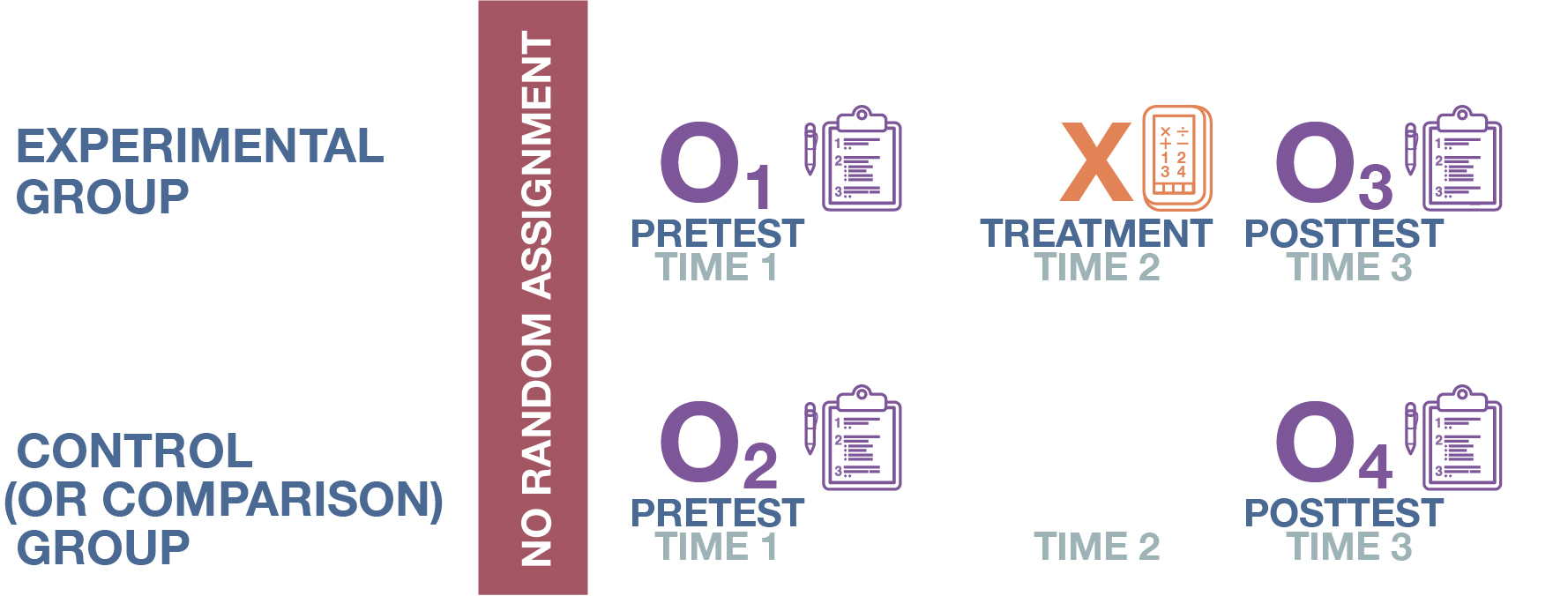
A nonequivalent control group design is the most commonly used quasi-experimental design. As shown in Figure 12.10, this design basically amounts to a classical experiment without random assignment. Note that researchers may refer to their control groups as comparison groups when they use this design. The lack of randomization means they cannot be as confident that the two groups are as comparable as control and treatment groups are meant to be.

Researchers sometimes choose this option because similar groups already exist that can serve as control and experimental groups without the need to go through the trouble of randomization. By doing so, they create a major vulnerability (i.e., selection threat) in their study, but practical considerations may overrule that fear. Indeed, when we were considering the different experimental designs we could use to evaluate the AddUpDog math app earlier, we talked rather blithely about how we would just randomly select fourth-graders for our experimental and control groups. If we actually tried to conduct this experiment at an elementary school, however, administrators might very well reject this research design. They might tell us to provide the app to all the students in a particular classroom, and compare their test scores with those of students in another classroom.

While school administrators might see this as a much more practical strategy to implement, it ruins our neatly randomized design. For example, perhaps the students in the classroom we chose to be our treatment group happen to be more enthusiastic about extracurricular enrichment than the students in the classroom we chose to be our control group. They may score equivalently on our math pretest, but their greater willingness to use the app may make it more effective in their hands, exaggerating our estimate of the app’s ability to improve math skills for the general fourth-grade population. This selection bias is always a possibility when we can’t use randomization to ensure equivalent groups. Unless we can adequately account for all the relevant characteristics that might influence the dependent variable and also differ across our two groups, selection will remain a potential explanation for our results.

A similar quasi-experimental approach replaces random assignment with a matching procedure. Two kinds of matching are commonly used. Individual matching involves pairing participants with similar personal attributes. In the math app example, we could pair two students who exhibit a high appreciation for math. The matched pair is then randomly split, with one participant going to the experimental group and the other to the control group. We would continue with this process until we have enough participants in our two groups. In aggregate matching, researchers basically adopt a nonequivalent control group design, identifying a comparison group that is similar on important variables to the experimental group. Multiple pairs of treatment and comparison groups can be created in this fashion. For instance, in our AddUpDog evaluation, let’s say we give various fourth-grade classrooms a survey measuring their appreciation for math. Then we match two classrooms with high levels of appreciation, two more with moderate levels, and two more with low levels. Finally, we randomly assign one of the two classrooms at each level to the experimental group and the other to the control group.

In order to increase internal validity, researchers using matching procedures have to think carefully about which variables are important in their study, particularly when it comes to demographic variables or attributes that might impact their dependent variable. Those are the variables they will want to use for matching purposes. As you might have guessed, the downside here is that we need to know beforehand which variables are important. We are only able to match on characteristics that we know about. It is possible we might miss something relevant—such as the enthusiasm gap we noted earlier across a school’s fourth-grade classrooms. We might diligently match, only to find out later that we should have chosen other characteristics to ensure we had truly comparable groups. Randomization makes that task far easier, and choosing matching in its stead means we will always have to be on the lookout for possibly decisive differences in our groups. To their credit, quantitative researchers have developed sophisticated procedures to match cases based on multiple variables, creating propensity scores that quantify how similar cases are across those variables and automatically matching cases according to each one’s propensity score. At the end of the day, though, the essential problem remains that we need to make sure we have accounted for all the variables that might matter—all the possible confounders that might explain our results.

We should note here that longitudinal panel studies are sometimes described as quasi-experiments because they basically involve matching, too. When we have data over time on the same individual, we can see if their outcomes change because of the introduction of the independent variable—say, if their income increases after attending a training program. The person before the treatment is essentially our control group, and the person post-treatment (after going through the training) is our experimental group. The longitudinal design rules out many alternative explanations for the observed changes in the dependent variable because we’re looking at the exact same person. This is why sociologists are more confident about making causal arguments when they have longitudinal rather than cross-sectional data.

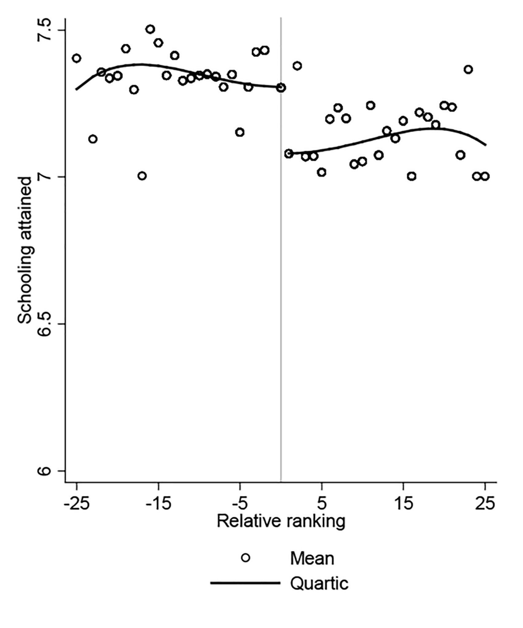
A more advanced type of quasi-experiment is a regression discontinuity design. In this approach, researchers choose their treatment and control groups from cases clustered around a “cut-off” point (a discontinuity) in a particular variable that determined whether the treatment was given. To give you a sense of what this technique entails, consider a study conducted by the World Bank, an intergovernmental organization that provides financing to lower-income countries pursuing development projects. World Bank researchers Deon Filmer and Norbert Schady (2009) wanted to evaluate whether a program that provided scholarships to at-risk children in Cambodia actually improved their school enrollment and attendance. They had data on the children who received the scholarship and those who didn’t, but they obviously couldn’t just compare school enrollment and attendance across the two groups, which differed on a variety of characteristics that could themselves explain any divergences in those outcomes. Furthermore, the program had not set up a lottery for distributing its scholarship (like the Moving to Opportunity experiment had done), which would have made measuring the impact of the scholarship more straightforward. That said, the sample of students available to them was so large that the researchers could pursue a regression discontinuity design. The program had given the scholarship to at-risk children, identifying them based on a “dropout risk score” they calculated using data on household characteristics and student test scores. What if researchers looked just at those students who were on either side of the cut-off for receiving the scholarship—those who scored right above and below the risk score threshold for eligibility? These students would be quite similar to each other, with a minor difference in their dropout risk score determining whether or not they received the scholarship. Thanks to their large sample, researchers were able to analyze outcomes just for those children whose dropout risk scores fell within a narrow 10-point band around the cut-off point. Within this fairly comparable group of students, they found that those children who received the scholarship had substantially higher school enrollment and attendance. You can see this striking discontinuity in Figure 12.11, where the vertical line shows a steep drop in educational attainment after students are no longer eligible for the scholarship.

You can appreciate why regression discontinuity designs require such large samples: researchers must focus their analysis on the cases clustered around the cut-off point while dropping many others. This design also requires a cut-off point that does not coincide with other important cut-offs (say, eligibility for other government programs) so that the participants on either side of that line are truly similar to one another except for the intervention of the stimulus.

With all the checks and balances provided by random assignment, the results of true experiments are much easier to defend than those of quasi-experiments—which detractors have dubbed “queasy experiments,” given the warranted fears that researchers should have about their internal validity. That said, regression discontinuity designs in particular have been shown to obtain similar results to studies using classic experimental designs. And for all their vulnerabilities, quasi-experiments have generated a great deal of compelling new research over the past few decades, enabling social scientists to study research questions that are tough or impossible to examine in a randomized controlled experiment. Indeed, an especially vibrant area of recent research involves natural experiments—quasi-experiments where the assignment of control and treatment groups is entirely out of the researchers’ hands.

Natural Experiments

Sometimes events in the real world happen to provide a researcher with novel ways to introduce features of experimental design into the analysis of observational data. In these particular cases, the researcher has no control over the event itself, which could be anything from a natural disaster, to a change in the weather, to the enactment of a new government policy. The key thing is that the occurrence of the event serves as a de facto “treatment,” changing the independent variable of interest. The researcher designs their study around the existing characteristics of the situation.

This sort of study is called a natural experiment. In this context, “natural” here does not mean the study has to involve a natural disaster (though a surprising number of social scientific studies do make use of hurricanes and the like for this purpose!). Rather, it indicates that the study’s researchers did not have control over the experiment. They did not themselves manipulate the independent variable. They could not create (artificial) conditions to precisely test the stimulus or treatment as they saw fit. This lack of control distinguishes natural experiments from interventional experiments. In fact, it’s probably more accurate to say that researchers “exploit” a natural experiment rather than “conducting” it. Conditions in the real world are changing on their own, and the savvy researcher is taking advantage of a very specific configuration of changes for their research purposes—sometimes long after the event transpired.

One of the most influential natural experiments in recent decades was a study by David Card and Alan Krueger (1994) of the effect of minimum-wage laws on employment. Before this study, economists had tightly held to the notion that any increase in the minimum wage—the lowest hourly wage that employers could pay their workers, by law—would generate greater unemployment. After all, economists theorized, employers would need to pay each worker more, and since they did not want to lower profits or raise prices—which would drive away customers—they would likely cut hours and lay off employees.

How could this theory be put to the test? Simply analyzing changes in employment after a state or locality decided to increase its minimum wage was fraught with problems, given all the possible alternative explanations we discussed earlier in the chapter. And for ethical and practical reasons, it was impossible to conduct a laboratory or field experiment that could persuasively assess this hypothesized causal relationship. Card and Krueger, however, decided to compare employment levels in two states—New Jersey and Pennsylvania—after New Jersey decided in 1992 to raise its minimum wage (from $4.25 to $5.05). In this natural experiment, New Jersey was essentially the treatment group, and Pennsylvania (which did not raise its minimum wage) the control group.

Card and Krueger narrowed their focus to make the comparison more akin to a true experiment. First, they obtained employment levels (measured by hours worked on a full-time basis) for fast-food establishments. Fast-food restaurants typically pay their workers the minimum wage, so these businesses should be most sensitive to any changes in minimum-wage laws. Second, the researchers collected data from a more restricted geographic area. Had they looked at statewide employment levels for New Jersey and Pennsylvania, the comparison would have been apples-to-oranges: any two states are very different in terms of their demographics and industrial makeup, which could be responsible for any observed differences in employment outcomes over time. To address this issue, Card and Krueger focused on fast-food establishments along the border of the two states, with the idea that the restaurants on either side of the border would be situated in similar communities whose main difference was which state policies affected them.

When Card and Kruger narrowed their analysis in these ways, they found that in the months before and after April 1, 1992—the day the minimum wage rose by 80 cents in New Jersey—fast-food employment rose in New Jersey but fell in Pennsylvania. These trends ran contrary to what prevailing economic theory predicted—that New Jersey should see a hit to employment after hiking its minimum wage.

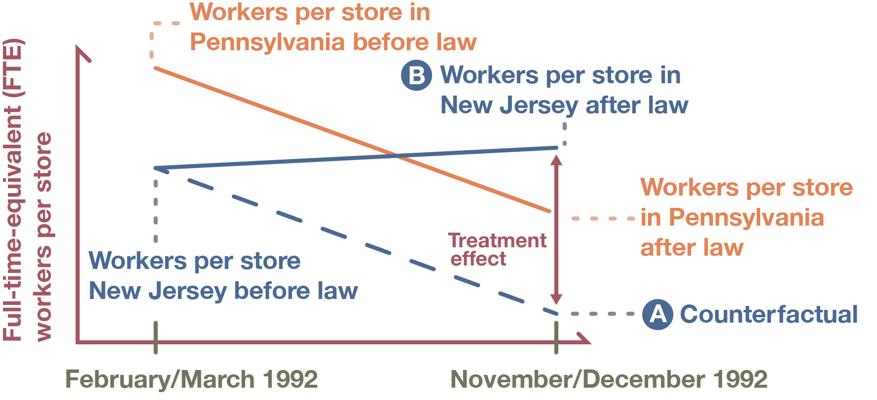
As we have discussed, however, a true experimental design assumes that the experimental and control groups are equivalent across all relevant characteristics except for the experimental group receiving the treatment. While comparing fast-food establishments across the border helped make the two groups comparable, there was still a substantial difference in employment levels between the two areas prior to the law change. New Jersey’s employment in the sector was actually lower than Pennsylvania’s during this earlier period. These different starting points—divergent pretest scores, essentially—needed to be accounted for. To do so, Card and Krueger employed a statistical technique called differences-in-differences (commonly used in studies exploiting natural experiments). As shown in Figure 12.12, the approach entails first calculating the change over time in the dependent variable for the treatment group (the treatment group’s “difference” over time) and then calculating the change over time for the control group (the control group’s “difference” over time). Then the two “differences” are compared (“differences in differences”). This technique accounts for the fact that the treatment and control groups did not start at the same place on the pretest. Had New Jersey not passed its minimum-wage law, its employment levels should have followed the downward path that Pennsylvania took, but starting from an even lower level. This counterfactual scenario, illustrated by the blue dashed line, dips down at the same angle as Pennsylvania’s employment does, landing at a point lower than where Pennsylvania arrived in the end (Point A). Therefore, a proper measure of average treatment effect—here, the impact of the minimum-wage increase on employment levels—would be the difference between that hypothetical scenario, the counterfactual (Point A), and what New Jersey actually experienced (Point B). When the researchers did that analysis, they found the increase in employment apparently caused by the minimum-wage hike to be even higher than the New Jersey trend by itself suggested.

Sometimes the “natural” intervention that researchers exploit in a natural experiment is exceedingly random and would seem to have little bearing on the dependent variable of interest—which is often the point, given the desire to avoid a selection effect. Sociologist David Kirk (2009) used a natural experiment to study whether people released from prison were less likely to return if they moved away from their former neighborhoods. The theory was that relocating would help break a parolee’s ties to friends and acquaintances involved with the sorts of criminal activity that had earlier landed the person in prison. Of course, a person’s housing decisions aren’t something that can be easily or ethically manipulated in a lab or field setting: we couldn’t, say, randomly choose some of the parolees to relocate and others to stay in their previous homes, and then track their recidivism (return to prison) rates. And if we wanted to just use observational data—say, comparing the recidivism rate of parolees who move after their release with those who do not—we would be concerned about the selection threat. Parolees who change their residence may be systematically different from those who do not—for instance, the movers may be more financially secure—and those differences themselves may make a return to prison more or less likely. In short, an observational analysis would not be able to adjudicate between the two causal stories here: that relocation actually made some people less likely to return to prison, or the two groups were just different to begin with.

Kirk found an ingenious natural experiment he could use to test his hypothesis connecting relocation to lower recidivism. Hurricane Katrina, a natural disaster that devastated New Orleans and other coastal areas in 2005, had leveled hundreds of thousands of homes. Kirk decided to study the recidivism rates of Louisiana parolees who were released in the period immediately following the destructive hurricane. If a parolee’s residence was severely damaged or destroyed, they had to move. Furthermore, the hurricane’s impact on parolees was random and had no relation to characteristics affecting their likelihood of recidivism. Therefore, parolees who had lost their homes could serve as a plausible treatment group for the study, capturing the effect of relocation without as great of a risk of selection. As an additional check, Kirk statistically controlled for multiple variables that could influence recidivism. (We’ll have more to say about how statistical controls can approximate control groups at the end of the chapter.) In line with his hypothesis, Kirk’s analysis found that parolees were significantly less likely to return to prison if they moved out of the parish.

To exploit natural experiments, researchers often need longitudinal data spanning the time before and after the event or policy change that serves as their treatment. For instance, Patrick Meirick and Stephanie Schartel Dunn (2015) wanted to see if Americans’ opinions about race changed as a result of Barack Obama’s 2008 presidential campaign. They focused on a series of events—the televised debates between the Democratic nominee and his Republican challenger John McCain—which, they argued, “gave tens of millions of Americans an extended look at a highly vivid, salient, cognitively available, counterstereotypical exemplar that may have changed the way they feel about African Americans.” As luck would have it, a telephone-recruited internet panel of the American National Election Survey (ANES) included a battery of questions about racial attitudes that they could use, and the panel had been surveyed multiple times that year, including in the months before and after the debates. Furthermore, the November survey asked respondents whether they had watched the debates, allowing the researchers to identify a comparison group of people who did not see the debates.

As you might be thinking, the natural experiment that Meirick and Dunn exploited was far from perfect. Among other things, their treatment and control groups were nonequivalent—we might expect non-debate watchers to be different from debate watchers on a host of characteristics. (To make the two groups more comparable, the researchers used statistical controls for demographic and party identification variables.) Nevertheless, the fortuitous availability of the ANES data and timing of the debates allowed the researchers to make a tidy comparison of pre-debate and post-debate racial attitudes. They concluded that watching the presidential debates led people to feel more positive affect toward African Americans across a range of explicit and implicit measures. However, the relationships were relatively weak.

As you can see across these examples, making use of a natural experimental design requires an ample amount of imaginative and versatile thinking. Researchers need to spot impactful (though possibly inconspicuous) developments in the world around them. They need to thoughtfully leverage those occurrences to identify treatment and control groups. And they often need to be exceedingly lucky, not just in terms of being around when the right disaster or policy change occurs, but also in terms of having access to data spanning the event in question. As daunting as this research endeavor can be, it allows researchers to investigate elusive connections between variables, extending experimental approaches to new domains while possibly avoiding the selection effects that routinely plague the analysis of observational data.

It’s also worth emphasizing how natural experiments are on the other end of the spectrum from lab experiments when it comes to experimenter control. Outside events determine the structure of the experiment, not the researcher’s own decisions. That means the researcher may find it difficult to comprehensively assess the effects (if any) of the treatment on outcomes—they may be stuck with whatever data happened to be collected. It also means that natural experiments are impossible to replicate: you’ll have to wait for another disaster to strike or another law to get enacted. We’re being a bit facetious here—clearly, one could design similar studies to test the same hypotheses—but replicating such a study is much harder than simply following a lab experiment’s methodological recipe. It is therefore harder to be confident that the results of natural experiments are not due to some fluke—however savvily that fluke was exploited for research purposes.

Deeper Dive: Time-Series Design

Earlier in the chapter, we noted how the absence of a control group posed major problems for an experiment’s internal validity, including the possibility that concurrent events could be responsible for observed changes (history threat) or the passage of time could lead to natural changes in outcomes (maturation threat). While creating a control group alongside the experimental group remains the best way to deal with these threats, to some extent they can be lessened by conducting several pretests and posttests over a longer period of time. We call this quasi-experimental approach—which has neither randomization nor a control group—a time-series design.

Let’s say that for whatever reason we cannot recruit a control group for our evaluation of the AddUpDog app—no child wants to miss the chance to touch (and tap) such technological greatness. We decide to use a time-series design as an alternative. As shown in Figure 12.13, we might decide to do four pretests before the students start using the app and then four posttests after they complete their 10 hours. How does this times-series design help us conduct a rigorous analysis of whether using the app improves math skills?

 

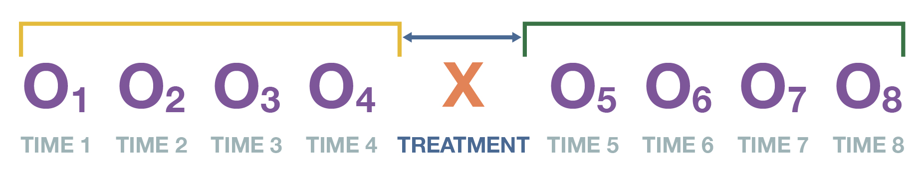
In comparison to just using one pretest and one posttest, this experimental design would give us a good sense of how stable the students’ scores were both before and after they used the app. Remember that a major threat to internal validity when we don’t have a control group is that other factors outside the experiment might account for abnormally high or low values on our experimental group’s pretest or posttest, which we could mistake for the effect of the treatment. With multiple pretests and posttests, these extraneous factors should not be as much of a concern, washing out across our many tests. Furthermore, this time-series design allows us to see whether the students’ posttest scores increased right after they used the app and whether they stayed high. If these two conditions are true, then we have some evidence that the app truly caused improvements in their math skills: the timing of the spike and its lasting effect both suggest a causal relationship. Figure 12.14 depicts what the trend lines would look like when the stimulus truly does have a causal effect.

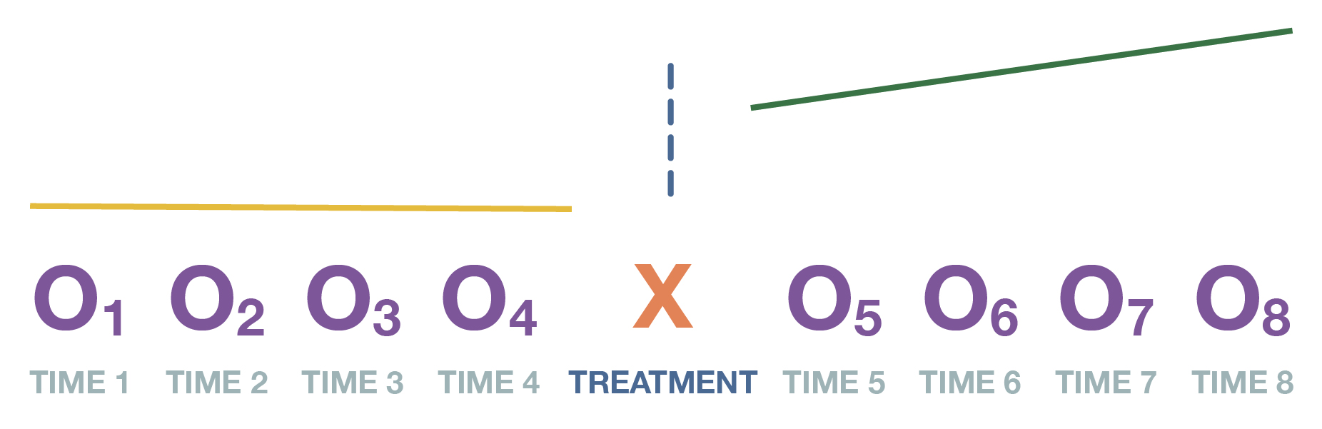
In short, what we’d like to see if our math app improves students’ test scores is some kind of clear discontinuity between the trend in scores before and after the stimulus. That pattern would suggest that the math app really did make a difference.

A time-series design has multiple observations of the dependent variable both before and after the introduction of the stimulus, but the exact number is up to the researcher—the more pretests and posttests, the clearer the trend lines become. With this design, the researcher can better understand the true value of the dependent variable before any experimental intervention. Likewise, the multiple observations afterward allow the researcher to compare the before and after trends in the dependent variable.

A study by sociologists Joseph Rodgers, Craig St. John, and Ronnie Coleman (2005) used a time-series design to test a set of social psychological theories that argued people had more children in response to natural disasters and disruptive political and cultural events. For their creative quasi-experiment, the researchers drew from birth-rate data immediately before and after the 1995 bombing of the Murrah Federal Building in Oklahoma City, a terrorist attack that killed 168 people, including 19 children. Their hypothesis was that local birth rates should have increased immediately afterward, consistent with the theoretical view that disasters—by drawing attention to people’s mortality—prompted them to hew to more traditional values and practices like having families and raising children.

When the researchers used advanced statistical techniques to graph their time-series data (shown in Figure 12.15), they saw a great deal of fluctuation in the trend line, as is typical for this kind of demographic data. Notably, while the fertility rate in Oklahoma County—where Oklahoma City is located—varied before the bombing (1990-early 1996), it seemed to vary around a relatively flat line. By contrast, in the period after the bombing (early 1996 to 1999), the fertility rate sloped upward. This discontinuity in the trend line suggested that the bombing did spur an increase in births, in line with social psychological theories.

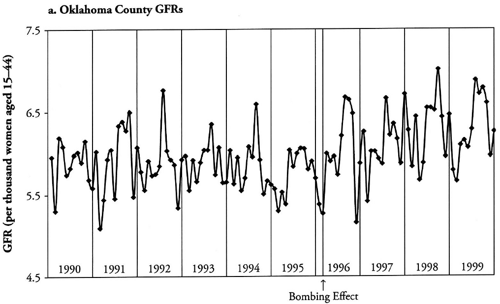
While a time-series design can be useful when a more rigorous experimental approach cannot be taken, it remains quite vulnerable to threats to internal validity. Even if the slopes of the trend lines we observe seem to confirm our hypothesis, we have to be wary about alternative explanations that have not been ruled out through the use of a control group and randomized assignment. For instance, while the post-bombing increase in Oklahoma County’s birth rate is striking, it may be the case that another event happening around the same time as the bombing was responsible for the increase (history threat). Or perhaps the fertility rate happened to be extraordinarily low in the period before the bombing and regressed to its mean afterward (regression threat).

Having a control group would strengthen any finding that the Oklahoma City bombing increased the fertility rate. But that was not possible in this retrospective study—and obviously, exposing people to trauma to see the effect on their decisions to have children is not ethical or feasible. However, it is possible to add one or more comparison groups to a time-series design, creating what is called a multiple time-series design. The approach is depicted in Figure 12.16.

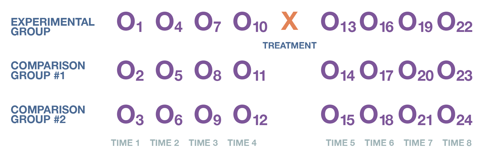
Rodgers and his collaborators decided to use a multiple time-series design to strengthen the internal validity of their study. How did they go about identifying comparison groups? They reasoned that if the theory connecting disasters to higher fertility were true, Oklahoma County, the county where the bombing occurred, should have experienced a higher increase in fertility afterward than other counties in the state did. Least able to tune out the horrifying consequences of the terrorist attack, Oklahoma City residents would have been the group most likely to follow through on the theory’s predictions of having more children. With this hypothesis in mind, the researchers used the other counties as comparison groups and saw how their fertility trend lines compared to those of Oklahoma County. They found that a baby boom appeared largely in and around the Oklahoma City area and persisted throughout the county, but the same dynamics did not hold elsewhere. Through the use of comparison groups, the scholars studying the Oklahoma City bombing were better able to support their causal argument that the disaster truly did lead to an increase in births.