14.1. Preparing for Data Analysis

Before you can begin any quantitative analysis, you need to place the data you wish to analyze into a dataset—a structured collection of data that is typically stored in one or more computer files (called data files). If you administered your own survey, you’ll need to enter the information from your survey forms into a new data file. If you’re using data that other researchers have collected (what we call secondary data), you will need to download the relevant data file or files along with any documentation that has been provided. In the following sections, we’ll go over these two approaches of creating a new dataset and using secondary data, respectively.

Creating a New Dataset

Whenever you administer a survey, it can be very exciting to receive those first few completed forms back from respondents. As the responses pile up, however, your emotions may shift from euphoria to dread. A mountain of data can be overwhelming. How can you pull a set of intelligible findings out of this stack of submitted forms?

One major advantage of quantitative methods such as survey research is that they enable researchers to describe large amounts of data, which can be represented by and reduced to numbers within a dataset. In order to condense your completed surveys into analyzable numbers, you’ll first need to create a codebook. A codebook is a document that describes the content, structure, and layout of your dataset and outlines how the researcher translated the data from words into numbers—a process we call coding. Note that the “coding” we’re doing here is different from the coding we do in qualitative data analysis. Even though both kinds of coding help us analyze our data, in this case we are not focused on deciphering and interpreting meanings from text or images. Coding of quantitative data tends to be more formulaic—a matter of converting people’s responses to survey questions (all or most of which were closed-ended to begin with) into numbers. The codebook records what specific response each of our numerical codes refers to.

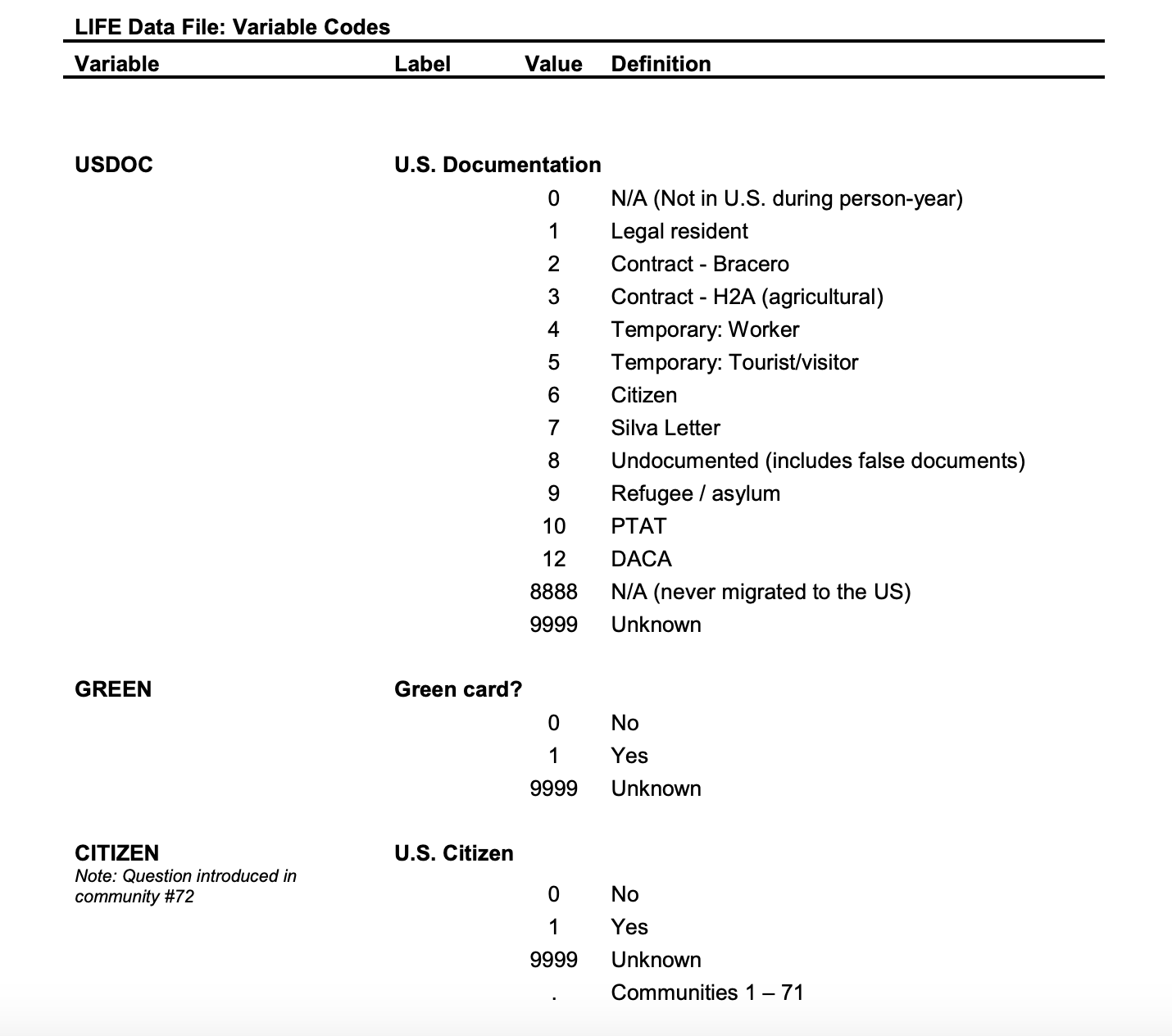
Codebooks can range from relatively simple to quite complex. Let’s discuss a fairly straightforward example of a codebook from the Mexican Migration Project, which has gathered data on the characteristics of migrants traveling from Mexico to the United States. As you can see in the codebook excerpt in Figure 14.1, the questions on the original survey (the survey items) have been converted into unique, single-word variable names. (As we’ll discuss later, the variable name comes in handy when entering data into a computer program for analysis.) In turn, the response options for each question (called attributes when they refer to different categories of a variable) have been converted into numerical values. For example, the two questions at the bottom—labeled with the variable names GREEN and CITIZEN—ask whether the respondent is a “green card” holder (i.e., a legally recognized permanent U.S. resident) and a U.S. citizen, respectively. For both questions, if the respondent answered “yes,” their response in the dataset was coded as 1; if they answered “no,” it was coded as 0. This codebook doesn’t contain the actual text for these two questions, but many codebooks will list the exact question wording after every variable name. Note that sometimes a survey item will have multiple variables attached to it—for instance, if the question allowed the respondent to choose multiple response options, which each need to be coded as a separate variable.

You may be wondering at this point why you should bother assigning numbers to simple response options like “yes” and “no.” One reason is that it makes entering data into your dataset easier. When it comes time to input a respondent’s answer into a data analysis program, you will just need to type “0” or “1,” rather than “yes” or “no” (or perhaps a much longer answer, depending on the specific response option). Coding responses in this way also reduces errors. For instance, if you typed in “nope” rather than “no,” your dimwitted computer will treat “nope” as a separate answer from “no.”

Note that in this example, there were only two response options given to respondents for each question: yes and no. When a variable only has two response options—yes/no, true/false, and so on—we call it a dichotomous variable. These two questions—captured in the two variables GREEN and CITIZEN—are a special kind of dichotomous variable: a dummy variable. For dummy variables, the code “0” indicates the absence of a condition and “1” indicates its presence. For the first GREEN question, then, “1” refers to green card holders, and “0” refers to everyone else (U.S. citizens, other visa holders, unauthorized migrants, and everyone else in the sample who does not have a green card) . For the second CITIZEN question, “1” refers to U.S. citizens, and “0” refers to everyone else—people who are not U.S. citizens. Researchers often prefer using this “0” and “1” coding scheme for simple dichotomous variables. Not only does it make certain kinds of advanced analysis easier, it also makes the interpretation of the variable very straightforward: “1” is always the presence of the condition listed in the variable name (for instance, a green card holder for GREEN, or a U.S. citizen for CITIZEN).

Following the example in Figure 14.1, you can create your own codebook in a word-processing document or spreadsheet. First, give each of your questions a unique variable name. Statistical analysis programs generally require the variable name to be a single word, so you will want to use something like GREEN or CITIZEN. If you need to use longer words or phrases, connect them with an underscore or just use abbreviations, such as PARTY_ID (for the political party a respondent identifies with) or POLORIENT (for their political orientation). As we noted earlier, codebooks often contain the full text of each question. so you can add it underneath the variable name. After the question text, you should list the question’s response options and the numerical codes you have assigned to each one.

Note that while your codebook contains your variable names, in an actual paper you will usually not want to list specific variable names (e.g., GREEN or CITIZEN). Those variable names only mean something to the researcher who is analyzing the dataset, so for public consumption, you generally just want to use a word or short phrase to describe the variable in the text: “the variable for permanent residency status” for GREEN, for instance, or “the variable for citizenship status” for CITIZEN. In special cases, researchers will mention variable names in a paper, and when they do so, they may choose to type out the names in all-caps (e.g., EDUC for education level) or in italicized lowercase letters (e.g., educ). We’ll follow the latter convention throughout the rest of the chapter so that you don’t think we’re shouting at you!

Your survey will likely be missing responses from some respondents on some questions. That’s okay. These nonresponses—what we call missing data—are unavoidable in large datasets. Respondents may not answer certain questions that are ambiguously worded or cover sensitive topics. They may accidentally skip a question—or even decide to give up on the survey altogether. During data entry, these nonresponses to questions should be categorized as missing values. (Missing values can be distinguished from valid values, data related to the actual response categories for your questions—in other words, the data you care about.) In your codebook, you can flag missing values by using a numeric value such as -1 or 99 that will not overlap with any valid values. For instance, if you are adding a question asking about a respondent’s age to your codebook, you probably wouldn’t want to use 99 as a missing value, since a person might very well have an age of 99. Instead, you’d want to use 999 or -1 since an age of 999 or -1 would be nonsensical in most contexts. (In the codebook excerpt presented in Figure 14.1, the value for missing data is 9999.)

Codebooks will frequently list two or more missing values for a question. That’s because in a survey interview a respondent may fail to respond in a particular way: they may refuse to answer a question, for instance, or they tell the interviewer, “I don’t know.” Rather treating these two non-answers as the same thing, you might want to create separate codes for each—say, giving “refuse to answer” a code of 98, and “don’t know” a code of 99.

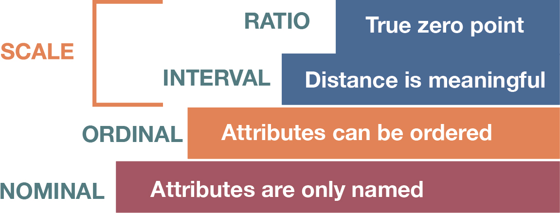
As you decide on how to code response categories, keep in mind the levels of measurement we discussed in Chapter 7: Measuring the Social World: nominal, ordinal, and scale. (These are illustrated in Figure 14.2, which appeared in that earlier chapter.) If you are using a scale-level variable, you may not need to provide codes for that variable in your codebook other than noting any missing values. For instance, if your scale-level variable was annual household income, and the respondent answered $60,000, the number 60000 could be stored as it is in your dataset, with no coding necessary. But what about for a nominal-level variable like the region of the country where a person lives? Which response category should be “1,” which should be “2,” and so on? Should any of them be coded as zero?

If you want to create a dummy variable out of your nominal-level variable, then, yes, you should use 1 for the region you want to highlight—say, the South—and 0 for everywhere else. Other than that specific yes/no scenario, though, the numbers you use don’t really matter for nominal-level variables. Figure 14.3A shows one possible scheme that includes five different U.S. regions (five response categories). In a straightforward fashion, they are numbered in alphabetical order.

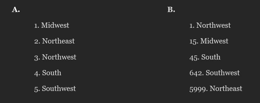
With a nominal-level variable like this, however, we could have gone with many other numbering schemes, including the one depicted in Figure 14.3B. For instance, we didn’t really need to list the different response options in alphabetical order, given that there is no intrinsic ordering to nominal-level attributes (the response options). That said, the first numbering scheme clearly looks better, and for your own sanity we advise arranging the response options in your codebook (and in your questionnaire) in a simple and logical fashion.

Next, let’s look at ordinal-level variables. Consider a question that the General Social Survey has asked in the past: “Do you believe there is a life after death?” This question could be answered in a variety of ways, and we might decide to simply provide our respondents with “yes” and “no” as response options. This question seems different, however, from the yes/no question we considered earlier that asked whether someone is a U.S. citizen. In this case, we might expect our respondents to have more or less intense beliefs about whether there really is life after death.

In their actual question, the General Social Survey captures this intensity of belief by using response options that collectively represent an ordinal-level variable. The coding scheme for this variable is shown in Figure 14.4A (note that the last two codes are missing values). In this example, the valid values are ordered by intensity: the higher the number, the weaker the respondent’s belief in life after death.

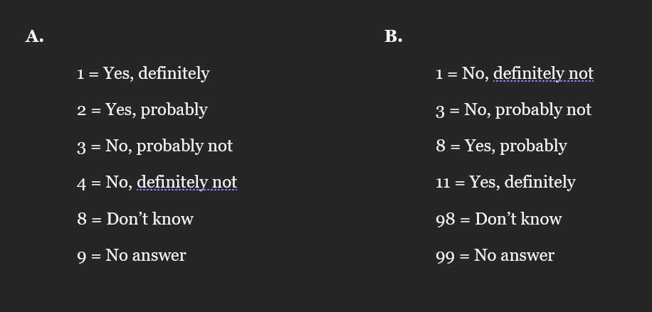
For ordinal-level variables, the rank order of any valid values should be clear. However, the GSS designers did not have to use the particular numbers in Panel A. They didn’t have to have a gap of just one integer between every pair of numbers, and they could have made those valid values track in the opposite direction, with higher numbers representing stronger belief—as shown in Figure 14.4B. Of course, using numbers with different-sized gaps between them seems unnecessarily complicated, and ordinal-level variables are typically represented by consecutive integers in datasets. The point here is that the codes you choose for these categories are somewhat arbitrary.

Once you’ve created your codebook, what’s next? If you’ve utilized an online tool such as SurveyMonkey to administer your survey, here’s some good news—most online survey tools come with the capability of importing survey results directly into a data analysis program. If you’ve administered your questionnaire in paper form, however, you’ll need to enter the data manually.

For those forced to conduct manual data entry, there probably isn’t much we can say about this task that will make you want to perform it other than pointing out the ultimate reward of having a dataset of your very own ready to analyze. At best, it is a Zen-like practice akin to raking sand. At worst, it is mind-numbingly boring. However, while you can pay someone else to do your data entry for you (a common chore given to student research assistants), you should ask yourself whether you trust someone else to make no errors in entering your data. Even a few typos can jeopardize the results of your project. It may be worth your time and effort to do the data entry yourself.

Secondary Data Analysis

Secondary data analysis is analysis of data that has previously been collected and tabulated by other sources. In this age of big data, where a vast and growing assortment of information has been digitized, you can find and download datasets on virtually any topic within minutes—many of them publicly accessible and free of charge. Government agencies at all levels routinely release data related to their operations—from city crime statistics, to monthly job reports from the U.S. Bureau of Labor Statistics, to country indicators of health and well-being compiled annually by the United Nations Development Program. In addition to the official data that governments release, you may also be able to obtain data from companies and organizations that conduct surveys or release selected portions of the data they generate about users and clients. Individual researchers frequently make the data they collected available to other scholars, too.

The main way that governments and other organizations provide their data is in an aggregated form—counts, averages, and other measures of anything from unemployment rates to the population’s gender breakdown, reported in tables and charts. While these figures can be useful, researchers often want to go beyond those aggregated results and look at the underlying data for themselves. They seek information on specific individuals (or whatever a dataset’s unit of analysis is). This microdata allows them to conduct their own analysis of patterns within variables and relationships between them.

Many government agencies and other organizations provide microdata in datasets they post online or otherwise offer to researchers, and this is the type of data you will want to obtain in order to do the analyses we cover in this chapter. We should also note that governments and other organizations routinely release data based on their own surveys, but occasionally they also allow researchers to examine administrative data—data from actual official processes, such as registration records and customer transactions, that organizations use for their operations. In the last chapter, for instance, we discussed how a team of sociologists was able to convince Michigan authorities to let them analyze records relating to people released from prison (Harding, Morenoff, and Wyse 2019). The use of administrative data has revolutionized the study of topics like income inequality. That’s because administrative data like tax records can provide much better estimates of people’s actual earnings than surveys do, given the problems with social desirability and accurate recall that we’ve previously discussed.

Especially if you are considering a quantitative research project, you should start by thinking about what datasets already exist on your topic. Have past surveys covered the concepts and relationships you want to examine? Have they sampled the target population you are most interested in? Would it be difficult for you to conduct your own survey that improves upon those prior efforts? If you are saying “yes” to all these questions, you will probably be better served using secondary data than doing your own data collection, which can be very costly in terms of time and money—especially when you need to generate a representative sample of large populations whose members are unknown to you.

Here are some of the key advantages of conducting secondary data analysis:

• You don’t have to spend time collecting the data. Analyzing secondary data enables you to avoid the entire data collection process, which can significantly speed up your research. All that’s required is that you have access to the data.
• You can find datasets very easily online. Government agencies typically share data with the public on their websites and in published form. Researchers will upload the datasets they analyzed for published work to online repositories or their professional websites. Frequently, a quick online search will locate relevant datasets for you to download. For example, a search for “adolescent risk behavior datasets” will lead you to the Youth Risk Behavior Surveillance System (YRBSS), a series of datasets compiled by the U.S. Centers for Disease Control and Prevention. Occasionally, getting access to a particular data file will require filling out online forms to identify yourself as a researcher and describe the study you are working on; less frequently, you may have to go through a formal process to apply for access (usually only for datasets with particularly sensitive personal information, such as health records). As we discuss later in the chapter, massive data archives also reside online, which you can search to locate datasets focused on very specific topics if a general web search turns up nothing. Finally, note that you can always ask an organization to share their data with you for research purposes. Sometimes, even corporations will share the microdata from surveys they conduct when the request has a scientific purpose.
• You don’t have to pay for most datasets. When governments collect data, they usually make the data files available for free. And when they fund studies, the conditions of the grant often require researchers to do the same. For instance, the General Social Survey, which we analyze later in this chapter, is funded by the National Science Foundation and can be downloaded for free. The majority of the thousands of datasets archived by the Inter-university Consortium for Political and Social Research (ICPSR) are free public-use files. The remainder can be downloaded by students, faculty, and staff at universities having memberships in ICPSR.
• You can find data from rigorously conducted surveys whose samples would be hard or impossible to obtain on your own. It is prohibitively expensive to survey large populations over wide geographic areas like a state or country. If you are conducting this research on your own, it is unlikely you’ll have the resources to generate a representative sample. You may want to leave it to the pros. Highly experienced survey specialists oversee major ongoing projects like the GSS, using sophisticated techniques to ensure their samples truly reflect the population of interest.
• You will not have to bother with getting institutional review board approval. Publicly available datasets are routinely anonymized, which means that researchers process the data to remove details that would allow individual respondents to be identified (see Chapter 8: Ethics for a discussion of the importance of protecting the identities of research participants). As a result, you usually do not need the institutional review board at your college or university to scrutinize the procedures of your study when you use secondary data (presumably, another institutional review board vetted the original survey). You will want to check with your institution to be sure.

As is true of all methodologies, there are also certain limitations to secondary data analysis:

• Organizations collecting secondary data may provide insufficient background information. You will not be able to evaluate the quality of the sampling or other data collection procedures a survey engaged in unless the original researchers did a good job of explaining their methodology. Government agencies that specialize in data collection, such as the U.S. Census Bureau, offer extensive information on the design and implementation of their surveys. So do well-respected research outlets like the National Opinion Research Center, Gallup, and the Pew Research Center. But a random one-off study may or may not have had rigorous procedures in place—you can look through the accompanying documentation to get a sense of their methods, but oftentimes you will be in the dark. Note that administrative data is likely to come with very little documentation because typically it was not meant for public consumption, which means you will need to make additional efforts to suss out the precise meaning of variables and response options or the organization’s specific procedures for data collection.
• You are limited to what questions have already been asked. This is a key reason that researchers choose to collect their own data: the available secondary data does not match their research purposes. If you want to research the factors that might influence a young woman’s decision to have a legal abortion, for instance, you would not want to look at the General Social Survey. That survey contains many questions about people’s attitudes about whether abortion should be legal, but it does not specifically ask how a respondent might approach that decision themselves. To pursue such a research question, you would need to find another survey that does a better job of measuring the relevant variables of interest—or you could field an original survey that asks the specific questions you want to ask.
• The secondary data available to you doesn’t measure what you want to measure in a valid way. This limitation is similar to the last point, but worth mentioning separately. Say that you would like to assess people’s attitudes about protecting the environment. You find a survey that does ask questions about the environment. However, it only asks respondents about climate change, recycling, and sustainable energy alternatives. These questions might be of interest to you, but unfortunately they could not provide you with a valid measure of a person’s overall attitudes about protecting the environment, which should go well beyond those three areas.
• Data may be in a different format than you require. For example, you might want to study young adults ages 18 to 25. However, you discover that the age variable in your secondary dataset is not measured in single years, but in ranges—and the first age category is 18 to 35. There is no way you could study your desired age range with that dataset.

If you decide you want to use secondary data, you can pursue two different strategies to find relevant datasets. One is to find questions on your specific topic within a survey that asks respondents about a wide range of topics (what is called an omnibus survey). A good place to start is the list of popular datasets we have collected at this site. Some ask general questions, while others have a narrower focus—for instance, on health or finances. Regardless, this search strategy is about identifying a relatively small set of relevant questions within an expansive survey questionnaire.

Note that some long-running surveys will regularly or occasionally have modules or supplements on specific topics. For instance, the General Social Survey asks many of the same questions every time it is fielded, but it will occasionally ask a set of questions about beliefs about science, views on the economy, or other topical issues just for that year’s survey. Browse a survey’s website to find out what modules or supplements it has done.

The second strategy for finding relevant secondary data is to search for a dataset focused more narrowly on your topic. In the data repositories section of our data page you will find a number of online catalogs where you can search for and download relevant datasets. The sidebar Searching a Data Repository has instructions on how to use the repository maintained by ICPSR, which stores datasets on a vast array of social-science topics.

Regardless of which strategy you take to find your dataset, eventually you should be able to get your hands on both the survey’s data files and its corresponding documentation. These should be available on the survey’s website or its page within a data repository. Frequently, a survey’s questionnaire is included or integrated within its codebook, though sometimes you will need to look for a separate questionnaire document in addition to the codebook (usually a PDF file). If it is available, you should download the version of the survey’s data file that is in a format matching whatever statistical software package you are using to analyze it (an SPSS dataset would have an SAV file extension, for example). If you can’t find the right format, it is possible to use the same data in another format. SPSS and other analysis packages can read data in the raw CSV (comma-separated values) used for simple spreadsheets, and you can also convert your data from one software package’s format to another’s.

Viewing a Quantitative Dataset

Regardless of whether you have fielded your own survey or are using data from someone else’s survey, at some point you will wind up with a dataset that you will need to analyze. Let’s use SPSS to open up a dataset from a national survey with thousands of respondents, the General Social Survey (GSS). The GSS is a national probability-sample survey that has been conducted since 1972—at first annually, but only every other year in more recent years due to budget cuts. (You can learn more about how the survey is conducted on its FAQ page.)

Datasets from any year of the GSS can be downloaded free of charge. We will be using the GSS from 2018 for all of the examples of data analysis in this chapter. Note that many of the variables we discuss are available in other years as well. If more recent datasets are available, or if you’d like to explore how the attitudes of U.S. adults have changed over time, you can repeat our analyses using the GSS data for other years.

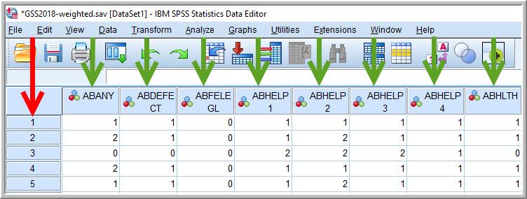
In SPSS, the GSS dataset you are analyzing will look something like the screenshot in Figure 14.5. Note that regardless of the analysis program being used, a typical dataset will be displayed with the units of analysis spread across the rows, and the variables spread across the columns. (Recall that a unit of analysis is the type of cases that a researcher is studying, which could be anything from individuals and households, to organizations and countries, to books and movies.) In the GSS dataset, each row represents an individual respondent, and each box (or cell) in the dataset represents how that respondent answered a particular question—specifically, the question measuring the variable listed at the top of the column for that cell.

In the dataset depicted in Figure 14.5, we see that Respondent #1 said “1” to the variable abany and “1” to abdefect. Respondent #2 said “2” to abany and “1” to abdefect. What do these numbers mean?

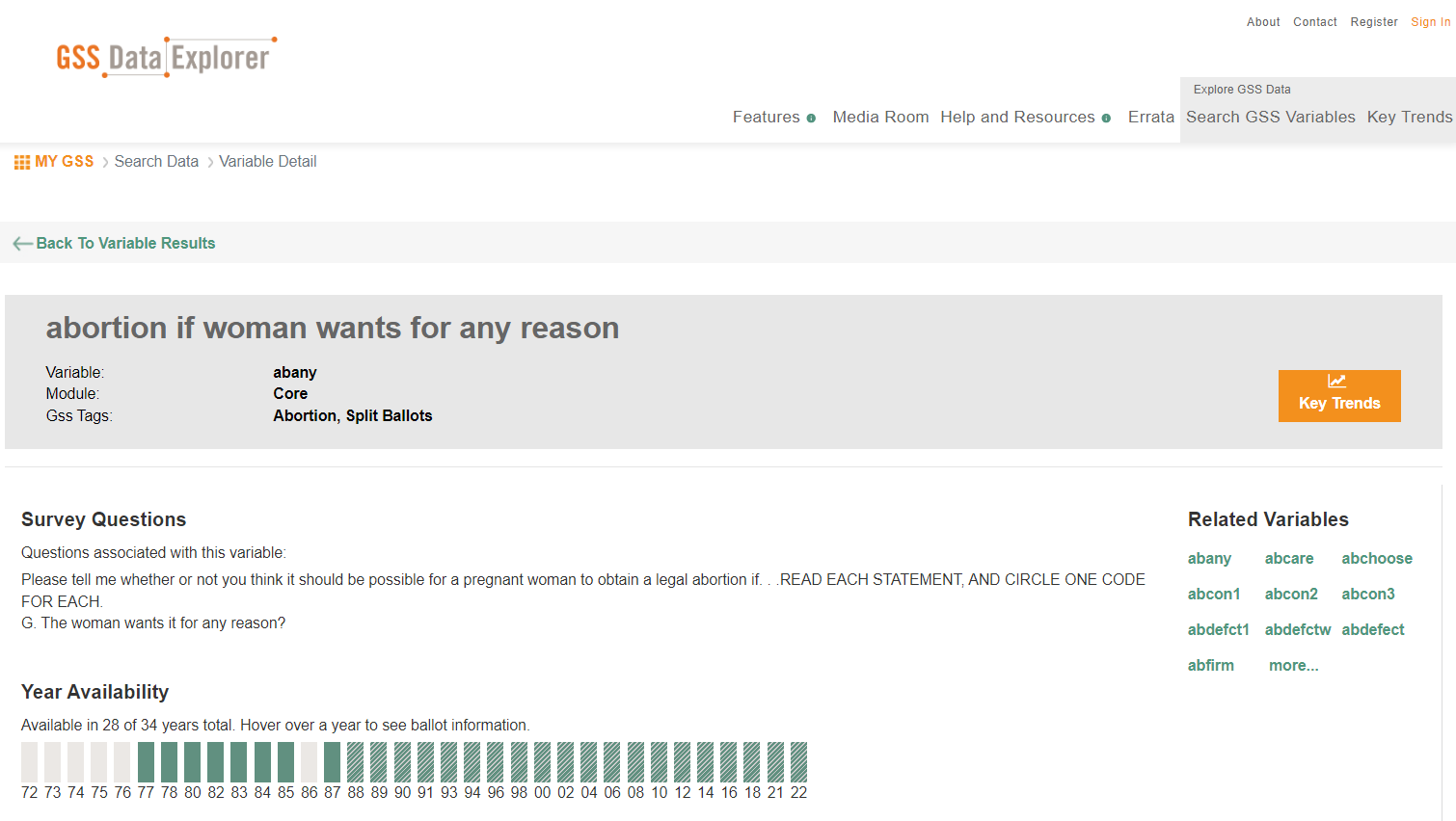
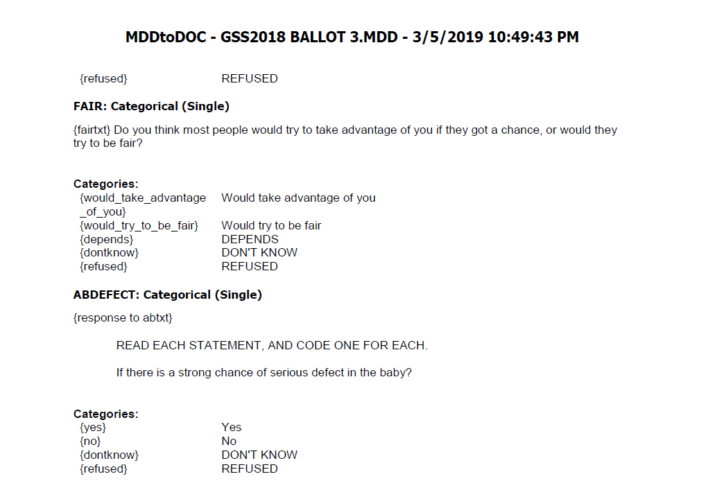
Remember that when entering survey responses into a dataset, you always enter them in numerical form—as codes. Furthermore, the questions are listed in the columns under their variable names. To know what questions go with particular variable names, and what response options go with particular codes, you’ll need to find documentation describing exactly which questions were asked to collect data for the GSS. You can either examine the codebook provided with the data or go to the Data Explorer on the GSS website, which allows you to look up variables and learn what questions they correspond to and in what years those questions were asked. (Other large surveys have similar online interfaces that can help you identify variables, though most of them force you to pore over their lengthy codebooks.) Figure 14.6 provides details about the abany variable taken from the GSS Data Explorer, and Figure 14.7 shows the entry in the GSS codebook for the abdefect variable.

Many secondary datasets include variable labels that summarize the questions, and value labels that tell you what response options the numerical codes reference. In a well-documented dataset, all the variables will be labeled (with variable labels) to represent the questions asked, and all the values of the survey’s ordinal- and nominal-level variables will be labeled (with value labels) to represent their response categories. Scale-level variables do not need value labels for their response categories, since the variable values are meaningful by themselves—say, a respondent’s age in years, or income in exact dollars.

The GSS dataset includes value labels for its response options, and it also includes variable labels with brief descriptions of each variable, but you should note that these variable labels do not include the entire text of each question. Remember that what exactly a variable measures depends on how exactly its corresponding question was worded, so you should get in the habit of always referring to the full question text rather than going by summaries. Furthermore, many datasets contain very little documentation, so the variable label and value label fields may be blank in your data file. You may want to add or edit these labels in your analysis program, using the questionnaire or codebook as a guide.

In SPSS, you can display the variable labels and other information about a dataset’s variables by clicking Variable View on the lower left of the screen. In Figure 14.8, we see the variable names in the far left column and information about each variable displayed in each row. Notice that under the Label column there’s a longer description of the abany variable: “Abortion if woman wants for any reason.” This variable label helps us a little bit, but we might still be wondering if abany refers to whether the respondent has ever had an abortion “for any reason,” or whether the respondent supports a woman’s right to have an abortion “for any reason.” If we look at the survey’s documentation (refer back to Figure 14.6), we learn that this is the complete question: “Please tell me whether or not you think it should be possible for a pregnant woman to obtain a legal abortion if the woman wants it for any reason?” (Remember: always look up the full text of the question!)

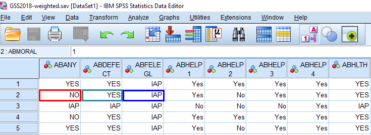
Because the nice folks who conduct the GSS also include value labels for response options when appropriate, you can view the datasets with those labels visible—making it easier to determine how exactly a given respondent (the rows in the dataset) responded to a particular question (the columns). When value labels are set, SPSS can instantly swap the numerical codes for each respondent’s answers with their corresponding value labels, as shown in Figure 14.8. With these labels displayed, it’s easy to see that Respondent #2 (second row) said “NO” to the variable abany and “YES” to abdefect. Referring back to Figure 14.5, which didn’t have value labels displayed, we see that the 2 for albany means “No” and the 1 for abdefect means “Yes.”

By the way, the value label “IAP” that you see under the abfelegl variable means that Respondent #2 was not asked that question. (abfelegl is yet another abortion-related question—as tipped off by the letters “AB” starting each of these variable names—and it asks if the respondent thinks “a woman should continue to be able to have an abortion legally or not.”) GSS employs a split-ballot design, which splits the overall sample into groups and uses a different set of supplementary questions for each group. In this case, the questionnaire (or ballot) that Respondent #2 received did not include the abfelegl question, so this person’s answer was marked as IAP, which stands for “inapplicable.” As you can see by referring back to Figure 14.5, IAP was numerically coded as 0.

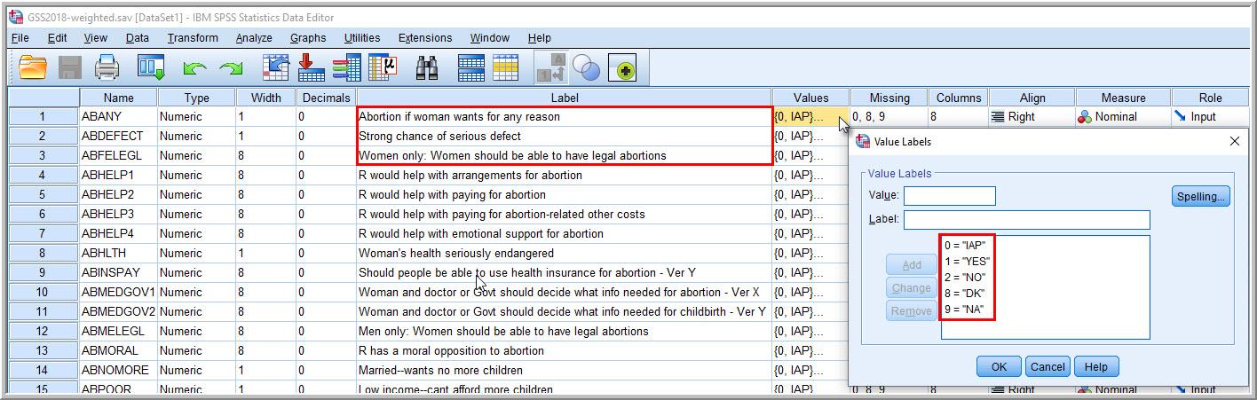
In a well-documented dataset, all the numerical codes for a particular variable will be listed, along with their corresponding value labels, in that variable’s entry in the SPSS Variable View window. (Make sure to click the tab on the bottom if you are currently in the Data View window.) If we click on the Values cell for a variable and then click on the three dots that appear on the right-hand side of the cell, a window opens up with the details for each response option. As Figure 14.9 shows, now we can see the numerical codes and associated value labels for abany in one place:

• 0 (IAP for “Inapplicable”)
• 1 (YES)
• 2 (NO)
• 8 (DK for “Don’t Know”)
• 9 (NA for “No Answer”)

To the right of the Values column in the Variable View window, note that there is a Missing column. By clicking on the cell under that column, we learn that albany has been assigned three missing values: 0, 8, and 9. These correspond to IAP (“Inapplicable”), DK (“Don’t know”), and NA (“No answer”), respectively. Since these three values are missing values, the other two values—1 (YES) and 2 (NO)—are our valid values for this variable. As we’ll describe in the next section, only valid values will appear in our analysis, and missing values will be excluded—which is what we want.